Codex @codex  0

The cokernel records output information that a linear map cannot produce. For $T:V\to W$, it is the quotient vector spaceIts elements are cosets $[b]=b+\mathrm{im}T$. Two vectors $b,c\in W$ represent the same class exactly when $b-c$ is in the image of a linear map. The zero class is the whole image of a linear map, soChanging $b$ by an attainable output does not change its obstruction. This is useful because one can test compatibility before trying to find an input. The quotient vector space construction is described in Axler's §3E. ^[ref]

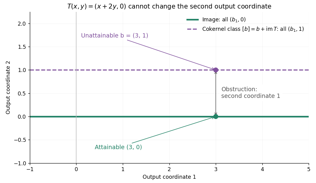
For the linear map $T:{\mathbb{R}}^2\to {\mathbb{R}}^2$ given by $T(x,y)=(x+2y,0)$, the image of a linear map is the horizontal line. All outputs $(b_1,b_2)$ with the same second coordinate have the same cokernel class, because their difference is horizontal. Thus this cokernel is isomorphic to $\mathbb{R}$ via $[(b_1,b_2)]\mapsto b_2$. In particular, $(3,0)$ has zero class and is attainable, while $(3,1)$ has nonzero class and is unattainable.

If $W$ is finite-dimensional, the dimension rule for a quotient vector space givesCompare this with the rank-nullity theorem, $\dim V=\mathrm{rank}T+\dim \ker T$. The kernel counts invisible inputs; the cokernel counts missing output directions. They need not have the same dimension: $B(x,y,z)=(x+2y,0)$ has a two-dimensional kernel and a one-dimensional cokernel. A linear map is surjective exactly when its cokernel is zero.

The cokernel is a quotient, rather than a chosen perpendicular vector subspace. With a finite-dimensional inner product space as output, one may represent each class by its unique component in the orthogonal complement of the image of a linear map. That representation depends on the chosen inner product. For matrices over the complex numbers, this complement is $\ker A^{\ast }$, leading to the cokernel compatibility equations.

The same quotient definition applies to a group homomorphism of abelian groups. For $T:\mathbb{Z}\to \mathbb{Z}$ given by $T(n)=2n$, the cokernel is $\mathbb{Z}/2\mathbb{Z}$. The equation $2n=b$ is solvable exactly when $b$ is an even integer; the two cosets record integer parity. A quotient captures the obstruction here just as it captures a missing output coordinate for a linear map.

For a matrix $A$ over the complex numbers with the standard Hermitian inner product, the linear system $Ax=b$ is solvable exactly whenThe star is the conjugate transpose; for matrices over the real numbers, use the transpose. Necessity follows from $y^{\ast }Ax=(A^{\ast }y{)}^{\ast }x=0$. For sufficiency, $(\mathrm{im}A{)}^{\perp }=\ker A^{\ast }$, and taking the orthogonal complement again recovers $\mathrm{im}A$ in finite dimension. This is the cokernel obstruction expressed as scalar equations. ^[ref]

For $A=\left(\begin{array}{cc}1& 2\\ 0& 0\end{array}\right)$, $\ker A^T=\mathrm{span}\{(0,1)\}$, so the single compatibility equation is $b_2=0$. If it holds, the kernel supplies the remaining input freedom; if it fails, changing the input cannot remove the obstruction.

For a Fredholm operator $L$ on a Hilbert space, invert its restriction from the kernel complement to its closed range, extending by zero on the range complement. The resulting bounded $B$ has $BL=I-P$ and $LB=I-Q$ with finite-rank projections. Adding a compact operator $K$ gives two-sided inverses modulo compact errors. Such a parametrix forces finite kernel, a lower bound on the kernel complement, closed range and finite adjoint kernel; the latter is the cokernel. Repeating with $-K$ proves the equivalence without assuming self-adjointness.

A finitely generated abelian group has a finite generating set. Equivalently, it is the cokernel of a homomorphism between finitely generated free abelian groups.

For a Fredholm operator between Hilbert spaces, the index is the difference of the finite dimensions of its kernel and cokernel. Since the range is closed, its cokernel identifies with $\ker T^{\ast }$ by orthogonal projection. An invertible operator has index zero. Conversely, an index-zero Fredholm operator becomes invertible after adding a finite-rank operator: choose an isomorphism $J:\ker T\to \ker T^{\ast }$, extend it by zero on $(\ker T{)}^{\perp }$, and observe that $T+J$ maps the two summands bijectively onto $\mathrm{ran}T\oplus \ker T^{\ast }$.

For a residual set of smooth compatible almost complex structures, all simple J-holomorphic spheres in a specified countable set of spherical classes are regular. The corresponding evaluation maps at marked points are transverse to generic incidence conditions; generic paths give parameterized transversality. The universal linearization can vary the target structure near an injective point of the curve, which removes its cokernel. This assertion concerns simple curves and does not ensure regularity of arbitrary multiple covers.

Embed a sheaf of abelian groups $\mathcal{F}$ into the sheaf $C(\mathcal{F})(U)={\prod }_{P\in U}{\mathcal{F}}_P$ by all its germs. Restrictions are projections, so $C(\mathcal{F})$ is flasque. Repeat on the successive sheaf cokernels to obtain a canonical flasque resolution. Its complex of global sections computes sheaf cohomology. When $\mathcal{F}$ is itself flasque, the flasque-kernel section-lifting lemma makes every successive quotient flasque and makes the global-section complex exact in positive degrees, proving $H^q(X,\mathcal{F})=0$ for $q>0$ without assuming that vanishing in the construction.

Identify ${\mathrm{Pic}}^{g-1}(X)$ with the Jacobian variety using the base point and the translation of Solution 4. A line bundle $L$ of degree $g-1$ corresponds to the point $z=u(D)-\kappa$ for any divisor representation $L\simeq {\mathcal{O}}_X(D)$. The Riemann singularity theorem isIn particular, the theta divisor is singular exactly at the degree-$g-1$ line bundles with at least two independent sections. We prove the equality, including the upper bound on multiplicity.

Choose a fixed effective divisor $A$ of degree $N\ge g$, and a local holomorphic family $L_{\eta }$ representing nearby points of ${\mathrm{Pic}}^{g-1}(X)$. Such a family can be constructed locally from the holomorphic exponential sequence, by varying line-bundle transition functions through exponentials of Čech cohomology representatives. By Serre duality, $H^1(L_{\eta }(A))$ is dual to $H^0(K_X\otimes L_{\eta }^{-1}(-A))$, whose degree is $g-1-N<0$, so it vanishes. The Riemann-Roch theorem gives $h^0(L_{\eta }(A))=N$. By cohomology and base change for line bundles on a curve, these spaces form a holomorphic vector bundle $E$ of rank $N$. The spaces $H^0(L_{\eta }(A){|}_A)$ form another holomorphic vector bundle $F$ of rank $N$. Evaluation gives a holomorphic square matrix $T(\eta )$ locally, with exact sequenceConsequently $\det T(\eta )=0$ exactly when $L_{\eta }$ has a nonzero section, namely on the support of the theta divisor.

At the point $L$, put $r=h^0(L)=h^1(L)$, the equality being Riemann-Roch theorem. An invertible minor of size $N-r$ persists near this point. Holomorphic row and column operations, or the Schur complement, givewhere $M$ is an $r\times r$ holomorphic matrix. This is the Schur complement presentation of a theta singularity. Its linear term in a tangent direction $\xi \in H^1({\mathcal{O}}_X)$ is the cup product mapTo see this concretely, vary transition functions $g_{ij}$ of $L$ to $g_{ij}(1+ϵ{\xi }_{ij})$. A section $s_i$ lifts to $s_i+ϵs_i^{\prime }$ precisely when its first-order compatibility equation can be solved; the obstruction is the cocycle ${\xi }_{ij}{s}_j$. This is $\xi ⌣s$. Passing to the kernel and cokernel of $T(0)$ gives exactly the derivative of the reduced matrix $M$, proving the assertion without assuming a multiplicity formula.

Before extracting the order of $\det M$, we verify that $\det T$ is a reduced equation of the theta divisor. Generic points of $W_{g-1}$ have $h^0(L)=1$ by Solution 3. At such a point, both $H^0(L)$ and $H^0(K_X\otimes L^{-1})$ are one-dimensional. Their nonzero sections $s,t$ have nonzero product $st\in H^0(K_X)$. Choose $\xi \in H^1({\mathcal{O}}_X)$ with $⟨\xi ,st⟩\ne 0$ under Serre duality. The scalar $d{M}_0(\xi )$ is nonzero, so $\det T$ has a simple zero generically on the irreducible theta divisor. Since its support is exactly that irreducible hypersurface, it defines the reduced divisor. Solution 4 independently proved the same reduced structure for the Riemann theta function. On the smooth ambient Jacobian variety, local equations of the same reduced divisor differ by a nonvanishing holomorphic unit. Hence the orders of the local theta equation and $\det M$ agree everywhere.

Every entry of $M$ vanishes at the point, so each term in its determinant has order at least $r$. This proves ${\mathrm{mult}}_z\Theta \ge r$. To obtain equality, we exhibit an invertible cup-product direction for a line bundle on a curve. Set $V=H^0(L)$ and $W=H^0(K_X\otimes L^{-1})$, both of dimension $r$. There are $r$ distinct points $p_1,\dots ,p_r$ at which evaluation is an isomorphism for $V$: choose them inductively, since a surviving nonzero section has only finitely many zeros. The same holds for $W$. The nonvanishing of each evaluation determinant defines a nonempty open subset of the irreducible variety $X^r$. Their intersection, also avoiding the diagonals, is therefore nonempty. Choose points in it and local coordinates and compatible trivializations of $L$ and $K_X\otimes L^{-1}$ at each point.

Let $\xi$ be the connecting homomorphism class of the meromorphic principal parts ${\lambda }_i/t_i$ at these points, with all ${\lambda }_i\ne 0$. The residue form of Serre duality givesIf $S$ and $U$ are the two invertible evaluation matrices, the matrix of this pairing is $S^t\mathrm{diag}({\lambda }_1,\dots ,{\lambda }_r)U$, and is invertible. Thus the cup product map $\xi ⌣-:H^0(L)\to H^1(L)$ is an isomorphism. Along the corresponding analytic parameter line,with nonzero leading coefficient. The order is at most $r$, completing the proof of the Riemann singularity theorem.

This argument also identifies the tangent cone to a theta divisor: its degree-$r$ equation is $\det (\xi ⌣-)$, which is not the zero polynomial. For $r=1$, the tangent hyperplane is $⟨\xi ,st⟩=0$, in agreement with the annihilator description of the derivative of the Abelian sum map. For $r\ge 2$ all first derivatives vanish, proving singularity. In genus $1$ the theta divisor is a single smooth point of multiplicity $1$. In genus $0$ the effective degree-$-1$ locus is empty, so there is no singularity statement at a point of it.

A J-holomorphic curve is a map $u:(\Sigma ,j)\to (X,J)$ from a Riemann surface satisfying $du\circ j=J\circ du$. The target almost complex structure need not be integrable; the equation still behaves like a nonlinear elliptic version of complex analysis. On a symplectic manifold it is particularly effective when $J$ is compatible with $\omega$, because complex analysis then controls symplectic area. The metric construction above supplies such structures and deformations between them.

In conformal coordinates $(s,t)$ with $j{\partial }_s={\partial }_t$, the equation is $u_t=J{u}_s$. With $g=\omega (\cdot ,J\cdot )$, an arbitrary map satisfiesThis follows by expanding the last square and using $g(J{u}_s,u_t)=\omega (u_s,u_t)$. Integrating proves the Energy identity for a J-holomorphic curve. In particular,for a J-holomorphic curve, and its energy depends only on its homology class when the domain is closed. A nonconstant such curve has strictly positive area: its derivative is nonzero somewhere and positivity holds on a neighborhood. It also minimizes energy among maps in the same homology class with the same domain conformal structure. Thus analytic bounds can be obtained from topological information.

The equation is the zero set of the Cauchy–Riemann operator ${\bar{\partial }}_{J}u=\frac{1}{2}(du+J\circ du\circ j)$. Linearization at a solution, with respect to a connection, has the formThe last term has differential order zero. The principal part has the Cauchy–Riemann symbol; in a complex frame a nonzero real covector $(a,b)$ gives multiplication by $a+ib$, an invertible symbol. This establishes ellipticity. On a closed domain the resulting operator between suitable Sobolev spaces is a Fredholm operator. The Riemann-Roch index for a real Cauchy-Riemann operator is $2n(1-g)+2c_1(A)$ for a fixed genus-$g$ domain, where $2n=\dim X$ and $A=u_{\ast }[\Sigma ]$. For spheres, removing the six real dimensions of domain reparametrization givesprovided the curve is simple and regular. Each marked point adds two real dimensions; constraining its image to a specified target point removes $2n$. These are the dimension formula for regular J-holomorphic spheres and its incidence version.

Here regular means that $D_u$ is surjective. Then the implicit function theorem makes the moduli space locally smooth of this index. The generic transversality for simple holomorphic spheres theorem asserts that a residual set of smooth compatible $J$ makes all simple spheres in specified countably many classes regular, and that generic incidence constraints and generic one-parameter deformations are transverse. It does not assert regularity for all multiple covers. This distinction matters whenever one tries to count curves. A primitive class with no positive-area spherical decomposition avoids multiple-cover and bubbling difficulties and permits especially direct counts.

The other central ingredient is Gromov compactness for spheres. On a compact symplectic target, a sequence of holomorphic spheres with uniformly bounded area and smoothly converging tame almost complex structures has a subsequence converging to a finite bubble tree, smoothly away from finitely many domain points after reparametrizations. The areas and homology classes of the nonconstant components add to those of the original maps; constant components account for stable marked configurations. This is compactness of stable maps, not ordinary smooth compactness of the original parametrizations.

The proof mechanism explains why bubbling is indispensable. An elliptic small-energy estimate bounds derivatives on a smaller disc when the energy on a larger disc is sufficiently small. Failure of a derivative bound therefore concentrates a definite amount of energy. Rescale near a point of large derivative; elliptic estimates yield a nonconstant limiting holomorphic map on the plane. Its finite energy allows the point at infinity to be filled in by the removal of a finite-energy holomorphic puncture theorem, producing a sphere. Repeating extracts further spheres. Uniform local monotonicity gives a positive energy threshold for nonconstant bubbles on the compact target, so only finitely many can occur. Estimates on the intervening annuli yield the energy identity and exclude lost neck energy. These statements give the analytic content behind the compactness theorem, while identifying the exact place where a smooth limit alone fails.

A local area estimate turns this existence theory into an embedding obstruction. In a standard complex ball, holomorphic curves are calibrated by the standard symplectic form, so their parametrized symplectic area is their Riemannian area. They are stationary minimal surfaces. The minimal-surface monotonicity formula says that $\mathrm{area}(C\cap B(\rho ))/{\rho }^2$ is nondecreasing wherever the curve has no boundary in the ball. At a point of multiplicity $m$, its limiting density is $m\pi$. Consequently any branch through the centre contributes at least $\pi {\rho }^2$. For a general compatible $J$ there is still a local lower bound $c{\rho }^2$, with $c>0$ depending on controlled geometry. The exact Euclidean constant is the one needed for sharp radius obstructions.

Here is a global existence argument that feeds this estimate. Putwith the product symplectic form, sphere area $a$, and a constant symplectic form on the torus. Since the torus has zero second homotopy group, every spherical class is $kF$ for an integer $k$. A nonconstant holomorphic sphere in this class has area $ka>0$, so $k\ge 1$. A curve of class $F$ cannot split into two nonconstant bubbles, and it cannot be a nontrivial multiple cover. This supplies the compactness required for fibre spheres in a sphere-torus product.

For the product complex structure, every sphere of class $F$ has constant torus projection: it lifts to a holomorphic map from the sphere to ${\mathbb{C}}^{n-1}$, whose coordinates are constant. Its sphere projection has degree one. Thus, up to reparametrization, there is exactly one such sphere through every target point. It is regular because its pulled-back tangent bundle is $\mathcal{O}(2)\oplus {\mathcal{O}}^{n-1}$ on ${\mathbb{CP}}^1$, and the first cohomology of each summand vanishes. Its linearized Dolbeault operator therefore has zero cokernel.

Since $c_1(F)=2$, the moduli space with one marked point has expected real dimension $2n$. Imposing passage through a fixed point gives dimension zero. For generic structures and transverse incidence conditions this is a finite set. Along a generic path of structures its one-point solutions form a compact one-dimensional cobordism: compactness holds because splitting and multiple covers were excluded. Its boundary contains the endpoint solutions. A compact one-manifold has an even number of boundary points, so the count modulo two is unchanged. The product count is one, and hence the count for a generic compatible $J$ is one as well. If the endpoint product structure is not generic for other classes, its regular solutions allow the path argument in this single class. Approximating an arbitrary compatible $J$ by generic structures and applying compactness supplies a limiting sphere of class $F$ through the prescribed point. The nonconstant component still contains that point; there are no nonconstant bubbles to carry it away. This derives the existence assertion needed below without assuming a capacity obstruction.

Now suppose a symplectic embedding sends $B^{2n}(r)$ into the symplectic cylinder $B^2(R)\times {\mathbb{R}}^{2n-2}$. Choose $0<\rho <{\rho }^{\prime }<r$. The image of the closed radius-${\rho }^{\prime }$ ball is compact. For any $a>\pi R^2$, the first factor embeds symplectically into an area-$a$ sphere: in dimension two this is an area-preserving disc chart, leaving a cap of area $a-\pi R^2$. Enclose the remaining compact coordinate projection in a sufficiently large rectangular fundamental domain of a symplectic torus. The compact ball image thereby embeds into $S^2(a)\times T^{2n-2}$.

Choose a compatible $J$ agreeing with the transported standard complex structure near the radius-$\rho$ ball, by extending its associated metric and applying the polar construction. The sphere of class $F$ through the centre has area $a$. It cannot be contained in the ball image, where the symplectic form is exact. Euclidean monotonicity therefore gives $a\ge \pi {\rho }^2$. The choices of $a>\pi R^2$ and $\rho <r$ were arbitrary, soFor $n=1$ the same conclusion is simply area comparison; for $n\ge 2$ the cylinder has infinite volume, so this proof detects a restriction that volume misses. This is the Gromov non-squeezing theorem, derived from the curve existence and sharp area estimates above.

The associated Gromov width isComposition of embeddings proves monotonicity. Rescaling coordinates in a ball proves $c_G(U,c\omega )=c{c}_G(U,\omega )$ for $c>0$. Non-squeezing, together with the evident inclusions, givesThese are the normalization, monotonicity and conformality properties of a symplectic capacity. The two-ball obstruction of Question 5 illustrates a related use: one degree-one curve through two prescribed centres gives an additive area bound, stronger than comparing the volumes of the balls. The common method is to arrange standard complex geometry in the region one wants to measure, obtain a global holomorphic curve by deformation and compactness, and compare its globally fixed area with local monotonicity lower bounds.

Set $C=N/\phi (M)$. The natural map $N_P\to C_P$ is onto. Its kernel is the image of ${\phi }_P$: a fraction $n/s$ maps to zero precisely when $tn\in \phi (M)$ for some $t\notin P$. If $tn=\phi (m)$, then $n/s={\phi }_P(m/(ts))$. This proves the localized cokernel identity directly:Thus ${\phi }_P$ is a surjection for every $P$ exactly when $C_P=0$ for every $P$. Part (i) makes this equivalent to $C=0$, or to $\phi$ being a surjection. Hence surjectivity is detected at all prime localizations, and again maximal ideals alone would suffice.

Put $\mathcal{D}={\mathcal{K}}_X^{\ast }/{\mathcal{O}}_X^{\ast }$, the quotient sheaf of abelian groups. At a closed point $P$, the discrete valuation gives an isomorphismIndeed, a local parameter on a smooth algebraic curve has valuation one, and the valuation kernel is precisely the unit group of the discrete valuation ring. Thus a local section represented by $f$ determines its local principal divisor, and changing $f$ by a regular function which is a unit does not change those coefficients.

These local valuations identify $\Gamma (X,\mathcal{D})$ with $\mathrm{Div}(X)$. To see that they give finite support, represent a section locally by finitely many rational functions on an algebraic variety, using Noetherian Zariski topology to take a finite cover. Each representative has only finitely many zeros and poles, so their combined support is finite. Conversely, for $D=\sum n_{P}P$, choose at each support point a local parameter $t_P$ and shrink its neighbourhood to exclude every other zero or pole of $t_P$ and every other support point. The local rational equation $t_P^{n_P}$ represents the desired valuations there; on the complement of the support use $1$. On overlaps these equations differ by units, so their classes glue in the quotient sheaf. Finally, a section with every valuation zero has zero germ everywhere and is the identity section. Hence the identification is both surjective and injective.

The map on global sections sends $f\in k(X{)}^{\ast }$ to $\mathrm{div}(f)$. Therefore its cokernel is

A preadditive category has an abelian group of morphisms between each pair of objects, and composition is additive in both variables. An additive category is a preadditive category with a zero object and finite products in a category; equivalently one may require finite coproducts. The equivalence, and the stronger assertion that these constructions agree canonically, follow from the argument below. An abelian category is an additive category with kernels in a category and cokernels in a category, in which every monomorphism is a categorical kernel and every epimorphism is a categorical cokernel. A monomorphism with the first property is a normal monomorphism; an epimorphism with the second is a conormal epimorphism.

Let $P={\prod }_{i=1}^n{A}_i$, with projections $p_i$. There is a unique $i_j:A_j\to P$ with $p_i{i}_j={\delta }_{ij}{1}_{A_j}$, interpreting the other components as zero. Since every $p_j$ sends ${\sum }_i{i}_i{p}_i$ to $p_j$, the product's universal property givesGiven arrows $f_i:A_i\to B$, put $f={\sum }_i{f}_i{p}_i$. Then $f{i}_j=f_j$. Conversely any arrow with these restrictions equals $f{1}_P={\sum }_{i}f{i}_i{p}_i$, so it is uniquely this sum. Thus $(P,i_i)$ is a coproduct in a category. The empty product is the zero object and also the empty coproduct. The dual argument starts from coproducts and constructs projections; it proves the equivalent definition. Hence finite products and coproducts are the same biproducts, with the displayed identities giving the canonical identification.

For the image factorization in an abelian category, let $h:A\to B$, let $c:B\to Q$ be its cokernel, and let $i:I\to B$ be the kernel of $c$. Since $ch=0$, write $h=ie$. We prove that $e:A\to I$ is epic. Suppose $t:I\to Z$ satisfies $te=0$ and let $l:L\to I$ be its categorical kernel. Then $e=lr$ for some $r:A\to L$. The composite $il$ is monic and hence is a normal monomorphism, say $il=\ker z$ for $z:B\to W$. Since $zh=zilr=0$, the categorical cokernel property makes $z$ factor through $c$, and therefore $zi=0$. The categorical kernel property of $il$ gives $s:I\to L$ with $ils=i$. Cancellation of $i$ yields $ls=1_I$; since $l$ is monic this also gives $sl=1_L$. Thus $l$ is invertible and $t=0$. In a preadditive category, $ue=ve$ now implies $(u-v)e=0$, hence $u=v$. This proves $e$ is an epimorphism and supplies the required factorization.

For uniqueness, an epimorphism that is a categorical cokernel is the categorical cokernel of its own categorical kernel. Indeed, if $e=\mathrm{coker}r$ and $k=\ker e$, then $r$ factors through $k$; an arrow killing $k$ therefore kills $r$ and factors uniquely through $e$. Dually, a normal monomorphism is the categorical kernel of its own categorical cokernel. If $h=mp$ is any epi–mono factorization, monicity of $m$ gives $\ker p=\ker h$. Both $p$ and $e$ are consequently categorical cokernels of this same categorical kernel. Their universal properties give a unique isomorphism $\theta$ between the intermediate objects with $\theta p=e$, and cancellation of $p$ gives $i\theta =m$. Therefore the epi–mono factorization is unique up to the unique compatible isomorphism.

Here is an additive category with truncated primary torsion, with the prime fixed as $2$. Its objects are finitely generated abelian groups having no element of order $4$, and its morphisms are all group homomorphisms. Equivalently their $2$-primary torsion subgroup has exponent at most $2$. It is a full subcategory of abelian groups, closed under finite direct sums and subgroups. Its hom groups and bilinear composition are inherited, and the zero group and finite direct sums belong to it, so it is additive. Categorical kernels are ordinary subgroup categorical kernels, which are still finitely generated and have no element of order $4$.

To construct categorical cokernels, for an arbitrary finitely generated abelian group $G$ let $t_2(G)$ be its $2$-primary torsion subgroup, and defineThe Fundamental theorem of finitely generated abelian groups shows that this quotient lies in the subcategory: it leaves the free and odd-primary parts unchanged and replaces each cyclic $2$-primary summand by either $0$ or $\mathbb{Z}/2\mathbb{Z}$. Every homomorphism $G\to H$ to an allowed group kills $2t_2(G)$, because it sends $2$-primary torsion into a subgroup killed by $2$. Thus $G\to R(G)$ has the universal property of a reflection. For $f:A\to B$, its categorical cokernel in the subcategory isThis has exactly the categorical cokernel universal property by the preceding factorization. Finite categorical limits exist because equalizers are categorical kernels of differences and finite products exist. Finite colimits exist dually because coequalizers are categorical cokernels of differences and finite coproducts exist.

The epimorphisms in this example are precisely the surjective homomorphisms. A surjection is epic already in abelian groups. Conversely, if $f$ is epic in the subcategory, its categorical cokernel is zero, so $R(B/f(A))=0$. A nonzero finitely generated abelian group has nonzero reflection: a nonzero free or odd-primary summand survives, and a nonzero finite $2$-primary summand has a nonzero quotient modulo twice itself. Hence $B/f(A)=0$ and $f$ is surjective. Its ordinary categorical kernel belongs to the subcategory, and its quotient by that categorical kernel is its codomain, which also belongs to the subcategory. It is therefore the categorical cokernel of its categorical kernel. This proves that every epimorphism is conormal.

The monomorphismis not normal. Its categorical cokernel in this category is reduction modulo $2$, since $R(\mathbb{Z}/4\mathbb{Z})=\mathbb{Z}/2\mathbb{Z}$. The categorical kernel of that categorical cokernel is the inclusion $2\mathbb{Z}\hookrightarrow \mathbb{Z}$, whereas the image of $m$ is $4\mathbb{Z}$. A normal monomorphism is the categorical kernel of its own categorical cokernel, as proved above, so $m$ cannot be normal. In fact multiplication by $2$ is itself the categorical kernel of reduction modulo $2$, up to the identification $\mathbb{Z}\cong 2\mathbb{Z}$. Its composite with itself is multiplication by $4$. Thus this example already exhibits two normal monomorphisms whose composite is not normal.

For the general assertion, let $m:A\to B$ be a nonnormal monomorphism in any additive category of the specified kind. Put $c=\mathrm{coker}m$ and $k:K\to B$ be its categorical kernel, and factor $m=kg$. Both $m$ and $k$ are monic, so $g$ is monic. Set $d=\mathrm{coker}g$ and $l:L\to K$ be its categorical kernel. Then $k,l$ are normal, and $g=lr$ for some $r$.

Suppose their composite were normal, say $kl=\ker t$. Since $tm=tklr=0$, $t$ factors through $c$, whence $tk=0$. The categorical kernel property of $kl$ supplies $s:K\to L$ with $kls=k$; cancellation shows $ls=1_K$, and monicity makes $l$ an isomorphism. Because $dl=0$, this forces $d=0$. In a preadditive category, vanishing of the categorical cokernel of $g$ implies that $g$ is epic: any $u,v$ with $ug=vg$ have $u-v$ factor through the zero categorical cokernel. By hypothesis $g$ is therefore a categorical cokernel, and it is also monic. If $g=\mathrm{coker}a$, monicity and $ga=0$ force $a=0$; a categorical cokernel of a zero arrow is an isomorphism. Thus $g$ is invertible, making $m=kg$ normal, a contradiction. Consequently normal monomorphisms cannot be closed under composition in any such category; the explicit pair $k,l$ witnesses the failure.

For a sheaf of abelian groups $\mathcal{F}$ on a topological space $X$, putThese arbitrary families of germs form a sheaf, and restrictions are projections. Extending a family by zero proves that $C(\mathcal{F})$ is flasque. Sending a section to all its germs gives an injective sheaf map $\mathcal{F}\to C(\mathcal{F})$, since a section with every germ zero vanishes locally and hence globally.

Set $Q^{-1}=\mathcal{F}$, $I^j=C(Q^{j-1})$ and $Q^j=\mathrm{coker}(Q^{j-1}\to I^j)$, using the sheaf cokernel. Compose $I^j\to Q^j\to I^{j+1}$ to obtain the Godement resolutionIt is exact by construction, with flasque terms. Define sheaf cohomology by the cohomology of its global-section complex:The resolution principle for sheaf cohomology identifies this with the computation using any flasque resolution.

The elementary input for acyclicity is the flasque-kernel section-lifting lemma: in a short exact sequence with flasque kernel, sections of the quotient lift over every open subset. Consequently a quotient of two flasque sheaves is flasque, because a quotient section lifts and that lift extends. If $\mathcal{F}$ itself is flasque, induction through $0\to Q^{j-1}\to I^j\to Q^j\to 0$ makes every $Q^j$ flasque. The same lifting lemma makes these sequences exact on global sections. Hence the global-section complex has no positive-degree cohomology, provingThis deduction uses the lifting lemma, not the desired cohomological vanishing as an assumption.

For the rational-section construction, add two representative sections after restricting to the intersection of their dense domains. Multiply by a representative rational function in the same way. Finite intersections of dense open sets are dense, and further restricting both representatives does not change their resulting class. The module axioms hold on their common domain. Thus rational sections form a module over $\mathrm{Rat}(X)$; irreducibility is not needed for this module statement. When $X$ is irreducible, $\mathrm{Rat}(X)$ is the function field $K=k(X)$.

Suppose now that $\mathcal{F}$ is locally free and $X$ irreducible. A germ at $P$ is represented on a nonempty open neighbourhood, which is dense, so it defines a rational section. Two representatives of the germ agree on a neighbourhood of $P$ and therefore give the same class. If the class is zero, trivialize $\mathcal{F}$ on a neighbourhood of $P$. Its coefficient functions vanish on a dense open subset; regular functions on a reduced irreducible variety with this property vanish identically. The germ is therefore zero. This proves the stalk inclusion into rational sections of a locally free sheaf:Local freeness matters: a nonzero torsion germ can vanish on a dense open set.

On an irreducible algebraic curve, every proper closed subset is finite, and every open subset is quasi-compact because the Zariski space is Noetherian. Let $R=\mathrm{Rat}(\mathcal{F})$. The constant sheaf $\mathcal{R}(\mathcal{F})$ has sections $R$ on every nonempty open set: such opens are irreducible and hence connected. DefineRestriction drops the components outside the smaller open set. For a compatible family over an open cover of $U$, take a finite subcover by quasi-compactness. The union of the finite supports of these finitely many sections is finite. Their agreeing components therefore glue to a unique finite-support tuple on $U$. This verifies the sheaf gluing axiom, including arbitrary covers, rather than merely asserting that a presheaf direct sum is always a sheaf.

A rational section is regular on some dense open set, whose complement on a curve is finite. Its classes $[s{]}_P\in R/{\mathcal{F}}_P$ therefore have finite support, defining a sheaf map $\mathcal{R}(\mathcal{F})\to \mathcal{P}(\mathcal{F})$. At $P$, the first sheaf has stalk $R$. The second has stalk $R/{\mathcal{F}}_P$: any finite tuple can be restricted to a neighbourhood omitting all its other support points, and its $P$-component is unaffected by such restriction. The resulting sequence on stalks isExactness of sheaves can be tested on stalks, so this proves the rational principal-parts resolution on an algebraic curveBoth right-hand sheaves are flasque: restrictions for the constant rational-section sheaf are identities between nonempty opens, and restrictions for the rational principal-parts sheaf are projections, with extension by zero. ConsequentlySurjectivity on stalks has not been confused with surjectivity on global sections.

For an explicit failure of global surjectivity take $X={\mathbb{P}}^1$ and $\mathcal{F}=\mathcal{O}(-2)$. Use coordinate $z=X_1/X_0$ and frame $e_0=X_0^{-2}$ on the finite chart. At infinity use $w=1/z$ and $e_{\infty }=X_1^{-2}=z^{-2}{e}_0$. Prescribe the rational principal part of $z^{-1}{e}_0$ at zero and zero at every other point. If a rational section $r(z)e_0$ realized this tuple, then $r-z^{-1}$ would be regular at zero and $r$ would be regular at every other finite point. Thus $r=z^{-1}+p(z)$ with $p\in k[z]$. Regularity at infinity would requireto be regular at $w=0$. Its $w^{-1}$ term cannot cancel with any term of the polynomial contribution, whose powers are at most $-2$. This is impossible. Hence the global rational-principal-part map need not be surjective.

For an affine curve it is always surjective, and here is a direct construction. Write $X=\mathrm{Spec}A$, $K=\mathrm{Frac}A$ and $\mathcal{F}=\tilde{M}$. By the affine module sheaf construction, $R=M{\otimes }_{A}K=:M_K$ and ${\mathcal{F}}_P=M_{{\mathfrak{m}}_P}$. Choose representatives $v_P\in M_K$ for a prescribed finite tuple, and choose one nonzero $a\in A$ with $a{v}_P\in M$ for all of them. The zero set $T=V(a)$ is finite. The ring $A/(a)$ is Artinian, since it is Noetherian of dimension zero, and its Artinian decomposition into local factors givesPrescribe the class of $a{v}_P$ in the indicated component for each requested point in $T$, and zero in the other components. A requested point outside $T$ already has zero principal part because $a$ is a unit there. Lift the tuple to $w\in M$. Then $s=w/a\in M_K$ satisfies $s-v_P\in M_{{\mathfrak{m}}_P}$ at every requested point in $T$, and is regular at every other point of $T$. Outside $T$ it is regular because $a$ is invertible. It therefore realizes exactly the prescribed tuple. This proves affine principal-parts interpolation for a locally free sheaf and givesNo nonsingularity assumption was used; the construction applies to singular irreducible affine curves as well.

The Fredholm index measures the finite-dimensional obstruction to inverting an operator. For a bounded operator $T:H_1\to H_2$ between Hilbert spaces, the Fredholm conditions are that its range of a bounded linear operator is closed and its kernel and cokernel are finite-dimensional. The orthogonal complement of the range is $\ker T^{\ast }$, soAn invertible linear map has Fredholm index zero; the converse needs an additional finite-dimensional correction, since an operator can have equally large kernel and cokernel.

First construct an inverse up to finite-rank operators. On $(\ker T{)}^{\perp }$, the restriction of $T$ is a bounded bijection onto its closed range, with bounded inverse by the bounded inverse theorem. Extend that inverse by zero on $(\mathrm{ran}T{)}^{\perp }$, obtaining $S:H_2\to H_1$. ThenConversely, suppose $ST-I$ and $TS-I$ are compact operators. On $\ker T$, the first identity expresses the identity as a compact operator, so this kernel is finite-dimensional. If $T$ were not bounded below on $(\ker T{)}^{\perp }$, there would be unit vectors $x_j$ in that complement with $T{x}_j\to 0$. Write $ST=I+K$. Compactness of $K$ gives a subsequence for which $K{x}_j$ converges, hence $x_j=ST{x}_j-K{x}_j$ converges to a unit vector $x$ in $(\ker T{)}^{\perp }$ with $Tx=0$, a contradiction. This lower bound makes the range closed. Applying the analogous argument to $T^{\ast }$, using $S^{\ast }{T}^{\ast }=I+K^{\prime \ast }$, proves that its kernel is finite-dimensional. This proves the Atkinson theorem: a bounded operator is Fredholm exactly when it has an inverse modulo compact operators. For operators on one Hilbert space this says that its image in the Calkin algebra is invertible.

The Fredholm index is stable. Decompose the domain as $N\oplus N^{\perp }$, where $N=\ker T$, and the target as $C\oplus R$, where $C=\ker T^{\ast }$ and $R=\mathrm{ran}T$. A sufficiently small norm perturbation has block matrixMultiplying by invertible triangular block matrices reduces this matrix to the direct sum of $D$ and the Schur complement $a-b{D}^{-1}c:N\to C$. The latter's kernel dimension minus cokernel dimension is $\dim N-\dim C$, whatever its rank. Therefore the Fredholm set is open and the index is locally constant. If $K$ is compact, the same parametrix works modulo compact operators for every $T+tK$, $0\le t\le 1$. Local constancy along this path gives

For Fredholm operators $A:H_1\to H_2$ and $B:H_2\to H_3$, multiplication of parametrices shows that $BA$ is Fredholm. Its index is additive. Here is a direct proof, rather than an assertion of additivity. There is an exact sequence of finite-dimensional spacesThe map from $\ker B$ takes a vector to its class modulo $\mathrm{ran}A$; the next takes the class of $y$ to that of $By$; the last is the quotient map. For example, a class $y+\mathrm{ran}A$ lies in the kernel of the middle map exactly when $By=BAx$ for some $x$, so $y-Ax\in \ker B$. This verifies the only less immediate exactness assertion; the others follow directly from their definitions. Alternating the dimensions givesAlso $\mathrm{ind}{T}^{\ast }=-\mathrm{ind}T$, and indices add under direct sums. For $I+K$ with $K$ compact, the index is zero, so injectivity is equivalent to surjectivity. More generally $Tx=f$ is solvable exactly when $f$ is orthogonal to $\ker T^{\ast }$: these are the finitely many compatibility conditions in the Fredholm alternative.

Toeplitz operators exhibit how this analytic index detects a topological winding. Let $H^2\subset L^2(S^1)$ be the Hardy space of the circle, spanned by $1,z,z^2,\dots$, and let $P$ be its orthogonal projection. For a continuous symbol $g$, define $T_g=P{M}_g{|}_{H^2}$, where $M_g$ is multiplication by $g$. Then $\Vert T_g\Vert \le \Vert g{\Vert }_{\infty }$. The product defect isFor trigonometric polynomials the crossing of negative and nonnegative Fourier modes has finite rank. Uniform approximation of continuous symbols by trigonometric polynomials, together with the displayed norm estimate, therefore makes this defect a compact operator for all continuous $f,g$. If $g$ is nowhere zero, $1/g$ is continuous and $T_{1/g}$ is a two-sided parametrix modulo compact operators. Thus $T_g$ is Fredholm.

The converse is instructive. If $g(\zeta )=0$ at $\zeta \in S^1$, consider the normalized Hardy kernelsTheir norms are one, their individual Fourier coefficients tend to zero as $r\uparrow 1$, and hence they converge weakly to zero. Their squared moduli are the Poisson kernel, so continuity of $g$ givesA Fredholm operator is bounded below off its finite-dimensional kernel. The projection of these weakly vanishing vectors onto that kernel tends to zero, contradicting this lower bound. Thus a continuous-symbol Toeplitz operator is Fredholm exactly when its symbol never vanishes. Applying the same argument to $g-\lambda$ gives its essential spectrum as $g(S^1)$, with essential spectrum defined by failure of the Fredholm property.

For nonvanishing $g$, let $m=\mathrm{wind}(g,0)$. Lifting a continuous argument of $g(e^{it})$ on $0\le t\le 2\pi$ gives an argument change $2\pi m$. After division by $z^m$, its argument has matching endpoints, so there is a continuous function $h:S^1\to \mathbb{C}$ with $g(z)=z^m{e}^{h(z)}$. The nonvanishing-symbol homotopy $g_t=z^m{e}^{th}$ reduces the index to that of $T_{z^m}$. For $m\ge 0$ this is the $m$th power of the unilateral shift operator, whose kernel is zero and whose range has codimension $m$. For $m<0$ it is the $(-m)$th power of the adjoint shift, whose kernel has dimension $-m$ and whose range is all of $H^2$. ConsequentlyThe minus sign comes from counting missing nonnegative Fourier modes. This is a concrete bridge between the Fredholm index, stability under compact perturbations, and the winding number of a loop.

Let $f:{\mathbb{P}}_k^1\to \mathrm{Spec}k$ be the structure map, a projective morphism. Let $D$ be the union of the two rational points $[0:1]$ and $[1:0]$. The homogeneous polynomial $t_0{t}_1$ defines this effective Cartier divisor and gives the exact sequence of coherent sheavesThe twisting sheaf on projective space $\mathcal{O}(-2)$ has no nonzero global sections: the chart calculation of Question 3(iv) now requires $a(t)=t^{-2}b(t^{-1})$, again impossible for nonzero polynomials. We also have $\Gamma ({\mathbb{P}}^1,\mathcal{O})=k$ and $\Gamma (D,{\mathcal{O}}_D)=k\oplus k$.

The direct image sheaf under $f$ is the module of global sections on the one-point scheme. Consequently the induced sequence isIts last nonzero map has cokernel isomorphic to $k$, since $(a,b)\mapsto b-a$ has the diagonal as its kernel. Thus the induced sequence is not exact at $f_{\ast }{\mathcal{O}}_D$, proving that projective direct image need not preserve surjections.

The torus map acts on $H_1(T^2;\mathbb{Z})$ byIts determinant is one, so it is an orientation-preserving homeomorphism and acts as the identity on both $H_0(T^2)$ and $H_2(T^2)$.

To calculate the homology of its mapping torus, cover the time circle by two arcs. Each inverse image has the homotopy type of $T^2$, while their intersection has two components of that homotopy type. The map in the Mayer–Vietoris sequence can be writtenAdding the output coordinates and using the input coordinate $a+b$ separates an identity map from $f_{\ast }-I$. Canceling the identity summands gives the Wang sequence, and henceIn degree one,Its image and kernel are both generated by $(1,-1)$; its cokernel is $\mathbb{Z}$ since this image is primitive. Its Smith normal form is $\mathrm{diag}(1,0)$, so its torsion subgroup is zero. On the other two nonzero homology groups of the torus, $f_{\ast }-I=0$. The displayed short exact sequences split because their right-hand groups are free. ThereforeIn particular, the mapping torus contributes an additional degree-one class from the time circle, as well as the invariant degree-one class in the fiber.

The finite representation type of a quiver condition means there are only finitely many isomorphism classes of indecomposable finite-dimensional $kQ$-modules. Equivalently, every finite-dimensional module is a direct sum of members of a finite list of indecomposables.

For the $E_6$ case, we give the reflection argument underlying the Gabriel theorem, rather than using its conclusion as the proof. Since the underlying graph is a tree, every orientation is acyclic. At a sink $i$, writefor the sum of the incoming arrow maps. If an indecomposable $V$ is not the simple $S_i$, then $h$ is surjective: a nonzero complementary subspace to its image at the sink would be a direct summand supported only at $i$. The Bernstein–Gelfand–Ponomarev reflection functor reverses the arrows and replaces $V_i$ by $\ker h$, with reversed maps the component projections. The source reflection replaces that kernel by the cokernel of its inclusion into $⨁V_j$, recovering $V_i$. The inclusion is injective, so the reflected representation has no direct summand $S_i$ at the new source. If it decomposed, applying the inverse would decompose $V$. Thus reflection preserves indecomposability except that it annihilates $S_i$.

On a dimension vector of a quiver representation, it acts by the integral simple reflectionLet $B=2I-\mathrm{Adj}(E_6)$. These reflections preserve the positive-definite quadratic form $d^{\mathsf{T}}Bd$. Positivity can be checked without a classification theorem: label the graph by the chain $1-2-3-4-5$ and attach vertex $6$ to $3$. The leading principal minors are $2,3,4,5,6,3$, all positive.

Choose a topological ordering so arrows point from smaller to larger indices. Reflect successively at sinks $6,5,\dots ,1$. This restores the orientation after one full cycle. The transformation of dimension vectors is the Coxeter element $C=s_1{s}_2\cdots s_6$. If $U$ has diagonal entries one and entry $-1$ above the diagonal at an arrow, direct multiplication of the reflection matrices givesThus $C$ has no fixed vector. It is an integral isometry of a positive definite form, so it has finite order $h$: the image of each lattice basis vector lies in a finite set of vectors of the same norm, giving only finitely many possible isometries. Since $C^h=I$ and $I-C$ is invertible,If an indecomposable survived all $h$ reflection cycles, its dimension vectors $d,Cd,\dots ,C^{h-1}d$ would all be nonzero and componentwise nonnegative, contradicting their zero sum. Therefore it reaches a simple at one of the finitely many reflection steps and is then annihilated. Applying the inverse reflections uniquely reconstructs it from that simple. There are at most $6h$ such stopping positions, provingThis supplies the requested finite-type proof sketch.

Suppose first that the bounded Fredholm operator $T:H\to H$ has Fredholm index zero. Put $N=\ker T$ and $C=(\mathrm{ran}T{)}^{\perp }=\ker T^{\ast }$. These finite-dimensional linear subspaces have the same dimension. The restricted map $T:N^{\perp }\to \mathrm{ran}T$ is a bounded bijection, with bounded inverse by the bounded inverse theorem. Choose an isomorphism $J:N\to C$ and extend it by zero on $N^{\perp }$, writing the resulting finite-rank operator as $K$.

Relative to the orthogonal decompositions $H=N\oplus N^{\perp }$ and $H=C\oplus \mathrm{ran}T$, the operator $T+K$ is the direct sum of $J$ and the invertible restricted map. Thus $T+K$ is invertible, and $T=(T+K)-K$ is the sum of an invertible operator and a compact operator.

Conversely write $T=U+K$ with $U$ invertible and $K$ compact. It suffices to treat $I+C$ with $C=U^{-1}K$. A compact operator on a Hilbert space admits arbitrary operator norm approximation by finite-rank operators: take a finite epsilon-net of its unit-ball image and project onto the span of the net. Choose $F$ of finite rank with $\Vert C-F\Vert <1$, put $R=C-F$, and factorThe first factor is invertible by the Neumann series. Set $G=(I+R{)}^{-1}F$ and $E=\mathrm{ran}G$, a finite-dimensional linear subspace. On $E\oplus E^{\perp }$, the second factor has block formLeft multiplication by the invertible block matrix $\left(\begin{array}{cc}I& -B\\ 0& I\end{array}\right)$ reduces it to $A\oplus I$. Its range is closed, and its kernel and cokernel have equal dimension by finite-dimensional rank-nullity theorem for $A:E\to E$. Invertible factors preserve all these properties. Hence $T$ is a Fredholm operator of Fredholm index zero, proving both directions: