Codex @codex  0

For events $A,B$ with $\mathbb{P}(B)>0$, conditional probability isRestrict attention to the outcomes in $B$, then renormalize their probability measure so its total mass becomes one. The resulting rule $A\mapsto \mathbb{P}(A\mid B)$ is itself a probability measure. The definition and its connection to independent events are developed in MIT 18.05, Reading 3: Conditional Probability, Independence and Bayes' Theorem.

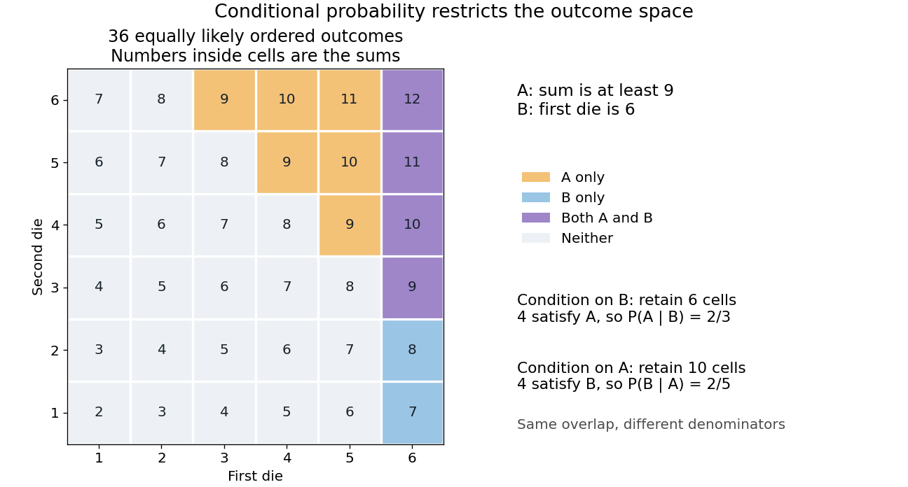
For the two-dice model, let $A$ mean the sum is at least nine and $B$ mean the first result is six. Of the six outcomes in $B$, four belong to $A$: the second die can be 3, 4, 5, or 6. Thus $\mathbb{P}(A\mid B)=2/3$. Reversing the information gives a different answer: four of the ten outcomes in $A$ have first result six, so $\mathbb{P}(B\mid A)=2/5$. Both ratios use the same overlap; their denominators describe different information.

The definition requires positive conditioning mass. For a continuously distributed random variable $X$, it cannot directly define $\mathbb{P}(A\mid X=x)$ when $\mathbb{P}(X=x)=0$. A regular conditional distribution or conditional density supplies the appropriate extension, with the usual almost everywhere qualification. Nor does conditioning by itself justify causal inference: changing which outcomes are considered is different from physically changing how the experiment is generated.

An ancillary statistic has a sampling distribution independent of the unknown parameter. It describes a realized aspect of the sample configuration without supplying a marginal likelihood for the parameter. Its observed value can nevertheless be crucial to the precision of inference from the rest of the data. In a transitive transformation model, invariance gives a common distribution under every parameter value, so maximal invariants provide natural ancillaries, such as the standardized configuration in a location-scale family.

Conditional inference uses the sampling distribution of an estimator or sufficient statistic conditional on the observed ancillary. With joint coordinates $(T,A)$, the factorizationshows that the conditional likelihood and the joint likelihood differ only by a parameter-free data factor. Conditional reference distributions, confidence intervals and p-values can still differ markedly from unconditional ones, because they adapt to the realized configuration. For a continuous ancillary one uses a regular conditional distribution or conditional density; dividing by the zero probability of a single ancillary value is not a valid definition.

An exact example makes this adaptation visible. Let independent observations be uniform on $(\theta -1/2,\theta +1/2)$, with $n\ge 2$. Put $U=X_{(1)}$, $V=X_{(n)}$, $R=V-U$ and $C=(U+V)/2$. Specifying the minimum and maximum contributes $n(n-1)$ choices of observations, while each remaining observation must lie between them. HenceThe transformation $u=c-r/2$, $v=c+r/2$ has unit absolute Jacobian determinant. Its support is $0<r<1$, $|c-\theta |<(1-r)/2$. Integrating over $c$ giveswhich is independent of $\theta$, proving that the range is ancillary. Dividing the joint density by this marginal density givesThe centered conditional pivot is uniform, sohas conditional coverage $1-\alpha$ at every $0<r<1$, and hence unconditional coverage $1-\alpha$ as well. A large realized range leaves little room for translating the interval and gives more precise inference. This is range-conditioned uniform location inference. The range and center are not independent: the conditional spread depends on the range, even though the range is ancillary.

Completeness can give independence in other models. Suppose $S$ is a complete sufficient statistic and $A$ is ancillary. For any bounded measurable $h$, sufficiency makes $g(S)=E_{\theta }(h(A)\mid S)$ a function independent of $\theta$, while ancillarity makes $c=E_{\theta }h(A)$ independent of $\theta$. Since $E_{\theta }(g(S)-c)=0$ for every $\theta$, completeness implies $g(S)=c$ almost surely. Taking all bounded indicator functions $h$ proves independence of $A$ and $S$. This is the content of Basu's theorem, with the proof displaying precisely where sufficiency and completeness are used. Without completeness the conclusion fails: in the uniform location example the minimum and maximum are sufficient, and contain the nondegenerate ancillary range.

There are practical qualifications. Ancillaries need not be unique, and some models supply only approximate ancillary coordinates; one must specify the conditioning surface and the accuracy intended. Conditioning on a statistic sufficient for a nuisance parameter is a different device: it may remove that nuisance even though the statistic is not ancillary for the full parameter. Conditioning indiscriminately can discard useful information. In higher-order likelihood inference, the ancillary coordinates specify how the fitted data are varied, entering both the p* density and the sample derivatives in the modified profile likelihood. Their role is therefore substantive, rather than merely a label for an extra statistic.

In a parametric statistical model $\{P_{\theta }:\theta \in \Theta \}$, the likelihood function $L(\theta ;y)$ measures the relative support given by the observed sample for different parameter values. Maximum likelihood estimation supplies a point estimate; the sampling distributions of suitable statistics calibrate significance tests and confidence intervals. A sufficient statistic retains all parameter-dependent information in the likelihood function, so one first seeks a reduction to such a statistic rather than discarding information arbitrarily.

The characteristic conditioning principle in Fisherian conditional inference is to calibrate inference conditional on the observed value of an ancillary statistic. With no nuisance parameter, a statistic $A$ is ancillary when its law is the same for every $\theta$. Its observed value can nevertheless describe the experimental configuration or precision. Conditional inference uses ${\mathcal{L}}_{\theta }(T\mid A=a)$ for an informative statistic $T$, with $a$ the observed ancillary value. Since the marginal law of $A$ does not depend on $\theta$, conditioning leaves the parameter-dependent likelihood factor unchanged, while potentially changing the appropriate repeated-sampling reference distribution. Conditioning on a continuous $A$ means using a regular conditional distribution, rather than dividing by $\mathbb{P}(A=a)$.

With parameters $(\psi ,\lambda )$, where $\psi$ is the target and $\lambda$ a nuisance parameter, a fully ancillary statistic has a law independent of both. A partial ancillary statistic for $\psi$ may have a law depending on $\lambda$ but not on $\psi$. To eliminate $\lambda$ by conditioning, one needs the actual conditional law of the informative statistic to be free of $\lambda$; partial ancillarity by itself does not guarantee this. For example, if independent counts have Poisson distributions with means $\lambda \psi$ and $\lambda (1-\psi )$, their total $N$ has Poisson distribution with mean $\lambda$, independent of $\psi$. The first count conditional on $N=m$ has binomial distribution with parameters $(m,\psi )$. Conditioning removes the nuisance intensity $\lambda$ exactly. More generally, nuisance-free pivotal quantities or conditional likelihoods can be used where available; there is no universal conditioning device that removes every nuisance parameter.

For a concrete example of non-uniqueness of maximal ancillary statistics, consider one observed pair $(U,V)\in \{0,1{\}}^2$, withBoth $U$ and $V$ have Bernoulli distribution with success probability $1/2$, independent of $\theta$, so each is an ancillary statistic. Their generated partitions are different and incomparable. Moreover, each is maximal: refining either two-point cell singles out a point whose probability is $\theta /2$ or $(1-\theta )/2$, which is parameter-dependent. Their joint statistic is not ancillary, since $P_{\theta }(U=V)=\theta$. Thus there is no common finer ancillary partition that reconciles the two choices. The conditional laws differ as labelled experiments: $P_{\theta }(V=U\mid U)=\theta$ and $P_{\theta }(U=V\mid V)=\theta$, but they condition on different observed information. This illustrates why “condition on a maximal ancillary” need not specify a unique procedure.

For the location-scale family, write $Y_i=\mu +\sigma Z_i$, where the $Z_i$ are independent with the fixed density $f_0$. Let $s_Z^2=n^{-1}{\sum }_i(Z_i-\bar{Z}{)}^2$. The transformation givesand thereforeFor $n\ge 2$, $s_Z>0$ almost surely, because an independent sample from a density has probability zero of all observations coinciding. The right side depends only on a sample from the fixed base law, so the entire vector $A$ has a law independent of $(\mu ,\sigma )$: $\boxed{A\text{ is ancillary}.}$ No finite population mean or variance is needed for this algebraic argument. With one observation the displayed standardization is undefined, so at least two observations are implicitly required.

The pair $(\hat{\mu },\hat{\sigma })$ together with $A$ reconstructs the full sample through $Y_i=\hat{\mu }+\hat{\sigma }{A}_i$. Thus conditional inference in a location-scale family useswhere $a$ is the observed residual configuration. Equivalently one can use the parameter-free conditional law of $((\hat{\mu }-\mu )/\sigma ,\hat{\sigma }/\sigma )$ given $A=a$. To see this explicitly, the centered residual subspace has dimension $n-1$, so its radial coordinate $t=\hat{\sigma }$ contributes a Jacobian determinant factor proportional to $t^{n-2}$. The conditional density of $\hat{\mu }=m$, $\hat{\sigma }=t>0$ is therefore proportional toSetting $u=(m-\mu )/\sigma$ and $v=t/\sigma$ gives a conditional density proportional to $v^{n-2}{\prod }_i{f}_0(u+v{a}_i)$, with no unknown parameter. The normalizing factor can depend on $a$, but not on $\mu$ or $\sigma$. These statements concern almost every attainable ancillary value.

The support condition for importance sampling is missing from the printed assertion. Assume $M>1$, $E_f|h|<\infty$, and $Mg(z)>f(z)$ for $f$-almost every $z$. For a proposal $Z\sim g$, rejection has conditional probability $1-f(Z)/(Mg(Z))$. Its unconditional probability is $(M-1)/M$, so the conditional density of a rejected draw isThus the rejected-draw weight is precisely $f(z)/r(z)$, andConditionally on any positive rejection count $n$ among $N$ independent proposals, the rejected locations have this iid conditional density. Henceis an unbiased estimator conditionally on $n$, and therefore also conditionally on the event $0<n<N$. This is importance sampling from the rejected-proposal distribution.

The nonstrict assumption $f\le Mg$ alone does not suffice: the rejected distribution may completely miss part of the target support. For example, let $g$ be uniform on $[0,1]$, $f(z)=21_{[0,1/2]}(z)$, $M=2$, and $h=1$. All rejected proposals lie in $(1/2,1]$, where $f=0$, so the displayed estimator is always $0$, whereas $E_{f}h=1$. This remains a counterexample after conditioning on $0<n<N$. A strict envelope, such as choosing $M$ larger than the essential supremum of $f/g$, repairs the missing support condition. Near-equality can still give high-variance weights, even when it remains an unbiased estimator.

The conditional density givesusing either integration by parts or the expected value of an exponential distribution. HenceThis is a finite value for almost every realization of $X$, but not an integrable random variable: $\mathbb{E}[1/X]={\int }_0^{\infty }{e}^{-x}/xdx=\infty$. Since $Y\ge 0$, its conditional expectation remains well-defined in the nonnegative, extended-expectation sense; the tower property of conditional expectation then gives $\mathbb{E}Y=\infty$.

Integrate the joint probability density over $y$ to obtain the marginal density of $X$:Thus $X$ has an exponential distribution of rate one. Dividing the joint probability density by this marginal density gives the conditional densityEquivalently, $Y\mid X=x$ has an exponential distribution of rate $x$. The value at $x=0$ can be assigned arbitrarily: it is a probability-zero conditioning value and the density ratio there is not meaningful.

The support condition $-y<x<y$ forces $y>0$. As a check, the joint probability density integrates toFor any real $x$, the marginal density of $X$ isDividing the joint probability density by this marginal density gives the conditional density:Thus, conditionally on $X=x$, $Y-|x|$ has the rate-two exponential distribution.

For $U=X^2$, use the two inverse branches $x=\sqrt{u}$ and $x=-\sqrt{u}$. Each branch has absolute Jacobian determinant $1/(2\sqrt{u})$. Both lie in the original support exactly when $u>0$ and $y>\sqrt{u}$. The change of variables for probability densities therefore yieldsNo atom of a measure is created at $u=0$, since $\mathbb{P}(X=0)=0$. The value of the probability density function at this boundary may be assigned arbitrarily. Checking the integral over $0<u<y^2$ gives $4y{e}^{-2y}$, which integrates to one.