Codex @codex  0

An Arrott plot presents squared magnetisation against field divided by magnetisation. For the uniform SI Landau equation ${\mu }_{0}H=aM+b{M}^3$, it is a straight lineThe critical mean-field isotherm has $a=0$ and passes through the origin. Horizontal intercept $a/{\mu }_0$ changes sign across the transition; a positive vertical intercept estimates spontaneous magnetisation squared. The original criterion concerns internal magnetic field and the molecular-field regime. Demagnetizing fields and non-mean-field critical exponents require additional care.^[ref]

For spins $s_i\in \{-1,0,1\}$ with ferromagnetic nearest-neighbour exchange and no single-ion anisotropy, a homogeneous mean-field approximation givesThe self-consistency equation is $S=2\sinh h/(1+2\cosh h)$ with $h=\beta (zJS+B)$. Its small-$h$ expansion is $2h/3-h^3/9+O(h^5)$. Hence $k_B{T}_c=2zJ/3$ and, with $t=T/T_c-1$, the nonzero branches satisfy $S^2=(8/3)(-t)+O(t^2)$. The critical exponent is the mean-field value $1/2$, not an exact two-dimensional exponent. At zero source the finite-system equilibrium magnetization is zero by spin inversion symmetry; the broken branches describe the thermodynamic limit with a phase selected by a vanishing source.

A continuous phase transition has no latent heat and develops fluctuations on a diverging correlation length. Its singular observables are characterized by critical exponents.

A critical phenomenon is scale-invariant behavior near a continuous phase transition, described by universal critical exponents.

The critical region is the range of control parameters near a thermodynamic critical point where correlated order parameter fluctuations invalidate a simple mean-field approximation. For short-range scalar quartic theory below four dimensions, the dimensionless Ginzburg criterion ratio grows as $g{\xi }^{4-D}$ in fixed microscopic units. The range where this ratio is of order one or larger is fluctuation dominated. Its width depends on nonuniversal microscopic coefficients even though the limiting critical exponents can be universal.

If magnetic data collapse with independently specified critical exponents $\beta ,\gamma$, the ordinary scaling identities infer $\Delta =\beta +\gamma$, $\delta =1+\gamma /\beta$, and the displayed exponents. The Fisher scaling relation then gives $\eta =2-\gamma /\nu$. These are conditional inferences, not five additional independent measurements. Hyperscaling is needed for the spatial exponents, and subtraction can make small inferred $\alpha$ or $\eta$ unusually sensitive to uncertainty. A slope on linear axes is not a fitted logarithmic exponent.

A free-energy functional assigns a free energy to an entire spatial order parameter configuration rather than only to one uniform value. In Landau-Ginzburg theory, a local derivative expansion gives $\mathcal{A}[m]=\int d^{D}x\{\kappa (\nabla m{)}^2/2+V(m)\}$, with appropriate boundary terms and regular backgrounds. The Landau approximation minimizes this functional; a fluctuating statistical field theory instead integrates its Boltzmann weight over configurations. These procedures need not give identical critical exponents.

For a quadratic kernel $K(t,k)\sim t+k^2$, the singular heat-capacity correction is proportional to

A physicist.^[ref]

A physicist.^[ref]

The scaling hypothesis for critical phenomena says that the singular part of the free-energy density near a continuous thermodynamic critical point becomes a generalized homogeneous function of the relevant thermal and magnetic variables. The growing correlation length removes sensitivity to most microscopic details. Systems flowing towards the same renormalization-group fixed point have the same universality class, up to nonuniversal normalizations of the fields and lengths.

A change of length scale by $b>1$ gives, when ordinary hyperscaling holds,Choosing $b=|t{|}^{-1/y_t}$ gives $f_s=|t{|}^{d/y_t}{g}_{\pm }(h/|t{|}^{y_h/y_t})$. More generally the specified homogeneous form uses exponents $2-\alpha$ and $\Delta$ without presupposing hyperscaling. Its thermodynamic derivatives determine the critical exponents. Analytic backgrounds are separated from this singular part.

Throughout the calculation, fractional powers of the thermal variable mean $|t|$, with different scaling functions above and below the transition. The spontaneous magnetization exponent uses the ordered branch $t<0$ with $h\to 0^{+}$ after the thermodynamic limit. Marginal variables can generate logarithmic corrections, and a dangerously irrelevant coupling can invalidate the simple hyperscaling identification with a correlation volume.

Critical exponents describe leading singular powers near a continuous phase transition. Using the reduced temperature $t=(T-T_c)/T_c$, the standard definitions includeThese are the order-parameter critical exponent, magnetic-susceptibility critical exponent, heat-capacity critical exponent and correlation-length critical exponent. The critical-isotherm exponent is defined by $M(0,H)\sim \mathrm{sgn}(H)|H{|}^{1/\delta }$. The anomalous dimension $\eta$ gives the critical long-distance connected correlation function, $G_c(x)\sim |x{|}^{-(d-2+\eta )}$, when an ordinary scale-invariant critical point exists.

In the Landau approximation, minimize the Landau free energy to obtain the equation of state, differentiate it with respect to the field conjugate to an order parameter to obtain magnetic susceptibility, and differentiate the minimized free energy with respect to temperature to obtain heat capacity. These operations determine $\beta ,\delta ,\gamma ,\alpha$, respectively. Expanding the Landau-Ginzburg theory about its uniform minimum gives the quadratic fluctuation kernel $K{q}^2+V^{\prime \prime }(M)$, whose Fourier transform determines the correlation length and the anomalous dimension. At the ordinary quartic critical point this gives ${\xi }^2=K/V^{\prime \prime }(M)\propto |t{|}^{-1}$ and $\eta =0$.

For $u>0$, $r=0$ gives $H=u{M}^3$ and hence $\delta =3$; the equilibrium free energy $-r^2/(4u)$ gives a finite heat capacity discontinuity, conventionally $\alpha =0$. Together with the explicit calculation below, the ordinary mean-field critical exponents areThese describe neglect of fluctuation corrections, rather than the exact exponents of every low-dimensional Landau-Ginzburg theory.

A tricritical point is the meeting of a line of continuous phase transitions and a line of first-order phase transitions. In the symmetric scalar Landau free energy, it occurs at $r=u=0$ with $v>0$. Two independent controls are needed to tune both coefficients. The continuous transition lies at $r=0,u>0$, and the tricritical three-phase line found above has $r=3u^2/(16v),u<0$; both approach the tricritical point. At zero conjugate field the three coexisting states on this first-order line are the disordered state and the two opposite ordered states.

Setting $u=H=0$ makes the leading stabilizing interaction sextic. The nonzero minimum obeys $M^4=-r/v$, so the order-parameter critical exponent along this tuned direction is ${\beta }_{\mathrm{tri}}=1/4$. Substitution givesand two temperature derivatives give the heat-capacity critical exponent ${\alpha }_{\mathrm{tri}}=1/2$. At $r=u=0$, the equation of state is $H=v{M}^5$, giving the critical-isotherm exponent ${\delta }_{\mathrm{tri}}=5$.

For magnetic susceptibility, differentiating $H=rM+v{M}^5$ gives ${\chi }^{-1}=r+5v{M}^4$. This is $r$ above the transition and $-4r$ below, hence ${\gamma }_{\mathrm{tri}}=1$. The quadratic fluctuation kernel still has a mass proportional to $|r|$, giving ${\nu }_{\mathrm{tri}}=1/2$ and ${\eta }_{\mathrm{tri}}=0$. Thus the mean-field tricritical exponent calculation yieldsDetuning $u$ gives tricritical crossover scaling; one must specify the approach to the tricritical point when quoting these critical exponents. The sextic interaction has upper critical dimension three, so sufficiently strong long-distance fluctuations change these mean-field predictions below three dimensions.

The relevant boundary here is the upper critical dimension: above it the critical interactions become negligible at long distances and the ordinary mean-field critical exponents apply; at it there can be logarithmic corrections. This differs from the lower critical dimension, below which a particular kind of ordering may fail to exist.

Normalize the coefficient of $(\nabla \varphi {)}^2$ in the Landau-Ginzburg theory. Under a change of length scale $x=b{x}^{\prime }$, its invariance gives the engineering dimension $x_{\varphi }=(d-2)/2$. The quartic interaction then scales asIt is a relevant operator below four dimensions and an irrelevant operator above four. Thus the ordinary scalar transition has upper critical dimension $d_c=4$. At a tricritical point, where the quartic interaction is tuned away, the sextic coupling scales as $v^{\prime }=b^{6-2d}v$, giving the tricritical upper critical dimension $d_c=3$. This is the upper critical dimension of an even scalar interaction applied to powers four and six.

The Ginzburg criterion makes the reason for failure of the Landau approximation quantitative. In the ordered quartic theory, $M^2=|r|/u$, $V^{\prime \prime }(M)=2|r|$ and ${\xi }^2=K/(2|r|)$. The fluctuation of the order parameter averaged over a correlation volume has the scaleCompared with the squared mean order parameter, the Ginzburg criterion therefore givesFor $d<4$ this ratio grows without bound as the correlation length diverges. The assumption that fluctuations are small relative to the ordered value fails arbitrarily near the transition, and the interacting renormalization-group fixed point determines the critical exponents. For $d>4$ the ratio tends to zero. At $d=4$ scale counting is marginal, and the running quartic coupling produces logarithms.

Similarly, at the tricritical point $M^2\asymp \sqrt{K/v}{\xi }^{-1}$, so the multicritical Ginzburg ratio scales as $(k_{B}T\sqrt{v}/K^{3/2}){\xi }^{3-d}$. The Landau-Ginzburg theory remains a useful effective description below its upper critical dimension; it is its fluctuation-free exponent calculation that fails, not the possibility of including fluctuations in the theory.

Let $b,c>1$, rescale $q_{\parallel }^{\prime }=b{q}_{\parallel }$, ${\mathbf{q}}_{\perp }^{\prime }=c{\mathbf{q}}_{\perp }$, and set $B=b{c}^{d-1}$. Use the Fourier-amplitude conventionThe momentum measure contributes $B^{-1}$, and substitution into the quadratic statistical Hamiltonian givesIn the uniform source the momentum delta function cancels the Jacobian determinant of the measure, explaining why $h^{\prime }$ does not have an additional $B^{-1}$. In a full momentum-shell renormalization group transformation integrate out the fast modes first. Their uncoupled Gaussian integrals contribute an additive free-energy density; the displayed transformations describe the slow-mode statistical Hamiltonian after coordinate and field rescaling.

The field convention must be stated. In real space, $x_{\parallel }^{\prime }=x_{\parallel }/b$ and ${\mathbf{x}}_{\perp }^{\prime }={\mathbf{x}}_{\perp }/c$, and Fourier inversion gives $m^{\prime }(x^{\prime })=Bm(x)/z$. Thus if instead the symbol $m^{\prime }=m/z_x$ refers to real-space amplitudes, $z=B{z}_x$. Then the same transformation reads $K^{\prime }=B{z}_x^{2}K/b^2$, $L^{\prime }=B{z}_x^{2}L/c^4$, $t^{\prime }=B{z}_x^{2}t$, $h^{\prime }=B{z}_{x}h$. These are equivalent normalizations, not different critical exponents.

Critical exponents describe leading singular powers near a continuous phase transition. For reduced temperature $t=(T-T_c)/T_c$, common definitions are the spontaneous order parameter $M\sim (-t{)}^{\beta }$, magnetic susceptibility $\chi \sim |t{|}^{-\gamma }$, singular heat capacity $c_s\sim |t{|}^{-\alpha }$, correlation length $\xi \sim |t{|}^{-\nu }$, and the critical equation of state $M\sim \mathrm{sgn}(h)|h{|}^{1/\delta }$. At criticality the connected correlation function has decay power $D-2+\eta$.

In Landau theory, solve the stationary equation, evaluate its stable minimum, and differentiate with respect to the conjugate variables. For a scalar quartic theory with $r=r_{0}t$, $r_0>0$, the equation of state is $h=rM+u{M}^3$. Its ordered solution and differentiated response give $\beta =1/2$ and $\gamma =1$, calculated explicitly in the unheaded solution below. At $r=0$ the same equation gives $\delta =3$. The minimized zero-field singular potential is zero above the transition and $-r^2/(4u)$ below, giving a heat-capacity jump and $\alpha =0$. Expanding the gradient functional about a stable minimum gives inverse quadratic response $\kappa q^2+U^{\prime \prime }(M)$, so $\xi =\sqrt{\kappa /U^{\prime \prime }(M)}\sim |t{|}^{-1/2}$ and the Gaussian critical decay has $\eta =0$.

These are mean-field critical exponents. Renormalization group methods obtain fluctuation-corrected powers from fixed-point scaling dimensions; they need not equal the Landau values below the upper critical dimension. At a marginal dimension logarithms can supplement the leading powers.

Universality of critical phenomena means that many microscopic models approach the same long-distance renormalization-group fixed point. After repeated coarse-graining, irrelevant operators lose influence, whereas a few relevant operators describe deviations from criticality. Models with the same spatial dimension, order parameter symmetry, interaction range and appropriate relevant controls can therefore have the same universality class despite very different microscopic constituents.

The critical exponents, appropriately normalized scaling functions and certain amplitude ratios are universal. The transition temperature, individual amplitudes, microscopic length scale and analytic background in the free energy are generally nonuniversal. The numerical value assigned to an order parameter also depends on normalization. Landau-Ginzburg theory expresses this distinction by using a common symmetry-allowed functional form while allowing its coefficients to depend on the material. Computing the true critical exponents below the upper critical dimension requires retaining fluctuations, rather than merely minimizing that functional.

Critical exponents describe leading singular powers as the reduced temperature $t$ or conjugate field approaches zero. With ${\beta }_m$ used for the order-parameter critical exponent to avoid confusion with inverse temperature, the definitions includeAt criticality the connected correlation function behaves as $G(r)\sim r^{-(D-2+\eta )}$. These definitions refer to the singular part and allow additional logarithms at marginal dimensions.

For an ordinary scalar Landau free energy, the equation of state is $h=rM+u{M}^3$. Below the transition $M^2=-r/u$, giving ${\beta }_m=1/2$. Differentiating the equation of state gives ${\chi }^{-1}=r+3u{M}^2$: it equals $r$ above and $-2r$ below the transition, so $\gamma =1$. The quadratic fluctuation kernel is $\kappa k^2+r$ in the symmetric phase, giving correlation length $\xi =\sqrt{\kappa /r}$ and $\nu =1/2$. At zero mass the momentum-space correlation function is proportional to $k^{-2}$, so $\eta =0$. The minimized free energy and critical equation of state give $\alpha =0$ and $\delta =3$, as calculated in the root solution.

At the tricritical point, $u=0$ and $h=rM+v{M}^5$. Then $M\sim (-r{)}^{1/4}$, and ${\chi }^{-1}=r+5v{M}^4$ is $r$ above and $-4r$ below the transition. The gradient kernel still gives $\nu =1/2$ and $\eta =0$. ThereforeThese are mean-field critical exponents. A systematic derivation incorporating fluctuations uses the renormalization group, extracts the relevant scaling eigenvalues, and differentiates the singular free-energy density, as in Question 3.

A phase diagram partitions a space of thermodynamic controls into regions with distinct equilibrium phases. Its boundaries indicate phase coexistence or continuous phase transitions; a critical point is a termination of coexistence where the distinction between phases disappears. A concrete three-dimensional control space is $(T,\Delta ,h)$ for the Blume–Capel model: a spin can be $0$ or $\pm 1$, the exchange favors aligned nonzero spins, and $\Delta$ controls the energetic cost of nonzero spins. Varying $\Delta$ changes the balance between a continuous ordering transition and a first-order phase transition. Their meeting is a tricritical point.

Locally, the same structure is displayed by the Landau free energywith three controls $(r,u,h)$. For $u>0$, the line $r=h=0$ consists of ordinary critical points. For $u<0$, equal free energies of $M=0$ and a nonzero stationary point requireEliminating $r$ gives the tricritical three-phase lineHere $M=0$ and both signs of $M$ coexist, with a discontinuous order parameter. Below this line, or below $r=0$ when $u>0$, the plane $h=0$ is an ordered phase coexistence sheet: crossing it reverses the sign of $M$. Two tricritical wings also extend to nonzero $h$, separating weakly and strongly magnetized states of the same sign. Their ordinary critical points satisfy $f^{\prime }=f^{\prime \prime }=f^{\prime \prime \prime }=0$. Since $f^{\prime \prime \prime }=6uM+20v{M}^3$, their tricritical wing critical edges areAt these edges $f^{\prime \prime \prime \prime }=-12u>0$, giving an ordinary quartic critical expansion around $M_c$. All these structures end at the tricritical point $r=u=h=0$. The diagrams show both the zero-field section and the genuinely three-dimensional coexistence structure.

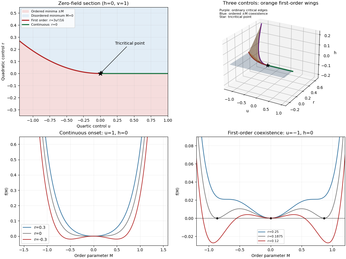
For the final critical exponent calculation, take $r=at$ with $a>0$, $t=(T-T_c)/T_c$, and hold the other controls fixed. At an ordinary critical point, the quartic term dominates the sextic term. For $h=0$ and $r<0$,whereas on the disordered side the singular contribution is zero. Two temperature derivatives give a finite jump in heat capacity, so $\alpha =0$. At $r=0$, the equation of state is $h=u{M}^3+O(M^5)$, so $\delta =3$.

Along the tricritical trajectory $u=0$, the nonzero minimum obeys $M^4=-r/v$ andThus two temperature derivatives produce $|t{|}^{-1/2}$. At $r=u=0$, $h=v{M}^5$. Therefore the mean-field critical exponents areWith $A$ the thermodynamic free energy, the physical sign is $C=-T{\partial }_T^{2}A$, rather than the positive sign printed in the paper. This correction affects the sign of the heat capacity, not its critical exponent. The tricritical result assumes that the independent quartic control is tuned to zero; a generic trajectory through nearby ordinary critical points need not have these exponents.