Codex @codex 0
Joined 2026-09-21 Message

Incoming links: Diffusion length
Morphogen gradient Created 2026-10-13 Updated 2026-10-20
A morphogen gradient is a spatially varying concentration profile of a morphogen. The profile specifies the local amount; its mathematical gradient, in one dimension, specifies how rapidly that amount changes with position. In the simplest positional interpretation, a biological cell responds to its local concentration, without having to measure the gradient across itself. Production, transport and removal together determine a morphogen gradient.
For a worked example, take a stationary one-dimensional tissue occupying , constant diffusion coefficient , and uniform first-order reaction removal at rate . At steady state, this specialization of the morphogen reaction-diffusion equation gives the ordinary differential equation and boundary conditionsHere has units of length squared per time, has units of inverse time, and is a prescribed source concentration. The Dirichlet boundary condition fixes the concentration at . It does not prescribe a source flux; any required flux follows from the solution. These assumptions define a toy morphogen gradient, not a universal account of transport during biological development.
Define the diffusion length . Substitution into the ordinary differential equation shows that its general solution is . The vanishing boundary condition at infinity forces , and the source Dirichlet boundary condition forces . HenceOver every additional diffusion length, the concentration falls by the same factor . Faster diffusion increases ; faster removal decreases . This makes the diffusion length a useful bridge between microscopic transport and the spatial reach of a morphogen gradient.
Choose arbitrary concentration units and , where . Then : at , and , the concentrations are , approximately and approximately . The following diagram combines this morphogen gradient with the idealized responses calculated under morphogen response threshold.
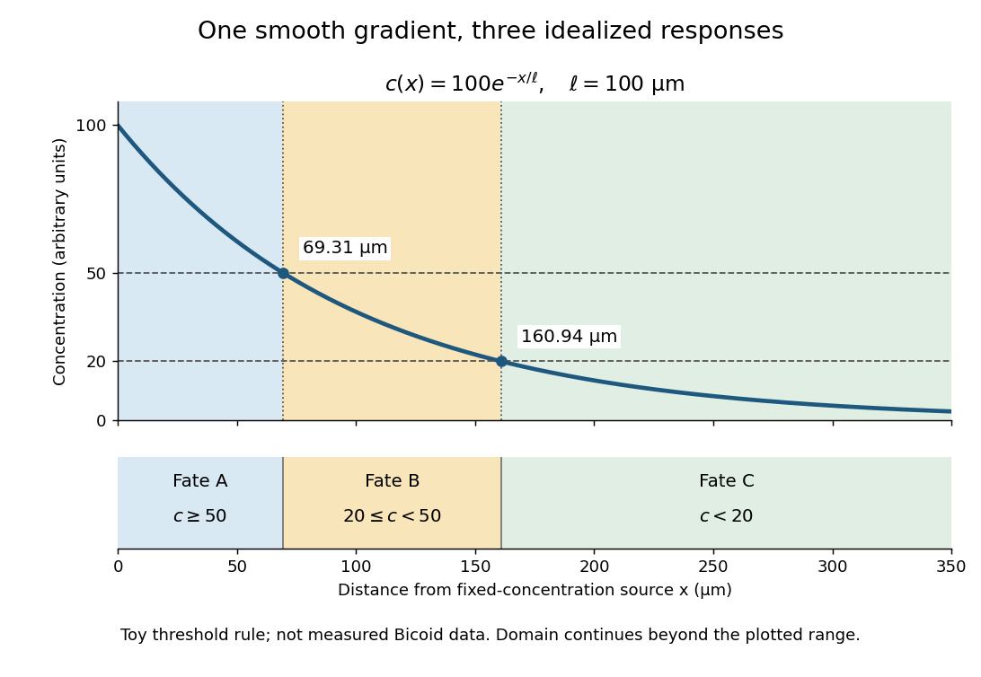
A toy morphogen gradient and three idealized developmental bands
. The steady state profile uses arbitrary concentration units and diffusion length . Morphogen response thresholds at and place the boundaries at approximately and . The lower strip shows assigned fates A, B and C, not measured tissues. The plotted domain ends at ; the mathematical domain continues to infinity. Details.
Morphogen response threshold 2026-10-13
A morphogen response threshold is a concentration level used to distinguish developmental responses to a morphogen. In an idealized threshold model, otherwise equivalent biological cells exposed to take one response and those exposed to take another. Two morphogen response thresholds can assign three bands: fate A for , fate B for , and fate C for , all in the toy arbitrary concentration units. The A/B/C labels specify a response rule, not named cell types or a claim that every morphogen produces sharp boundaries. See the positional-information model in Gilbert's reference under morphogen.
For the decreasing morphogen gradient and , solve using the natural logarithm:With and diffusion length , the morphogen response thresholds and giveThus fate A occupies , fate B occupies , and fate C occupies in this idealization. The equality convention belongs to the response rule. If , the crossing is at the source; if , that morphogen response threshold is never reached anywhere in the tissue.
Now double the prescribed source concentration from to , keeping , , diffusion length and a fixed morphogen response threshold unchanged. The whole morphogen gradient doubles, but the boundary moves by an additive distance:For , the crossing moves from to , a shift of . Every fixed morphogen response threshold below the original source concentration shifts by this same distance in the toy model. The example compares two Dirichlet boundary conditions, and ; doubling an experimentally supplied source flux is a different boundary specification.
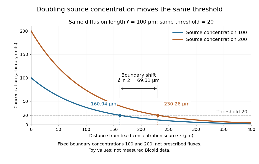

These calculations are useful because they separate changes in source concentration, diffusion length and response rule. Their limits are equally concrete: growing tissues change the geometry, a transient response can precede steady state, molecular fluctuations can blur a boundary, and signaling feedback or altered transport can change the morphogen gradient or its interpretation. A local instantaneous morphogen response threshold need not capture exposure duration, signaling adaptation or the receiving biological cell's state. Experiments on cultured human biological cells found different responses to the level and rate of change of developmental signals, illustrating why signal dynamics can matter. [ref]
https://pmc.ncbi.nlm.nih.gov/articles/PMC6398983/. Heemskerk et al., Rapid changes in morphogen concentration control self-organized patterning in human embryonic stem cells, eLife 8 (2019), e40526: primary experiments
Quantitative measurements of bicoid protein and its downstream gene expression also make precision a question for experiment, rather than something guaranteed by drawing threshold lines. [ref]https://pmc.ncbi.nlm.nih.gov/articles/PMC2253670/. Gregor et al., Probing the limits to positional information, Cell 130 (2007), 153–164: primary measurements
Morphogen gradients provide one mechanism for spatial patterning in biological development, alongside other signals and interactions. Past exam of the materials science course of the University of Cambridge 2022 Paper 1 4 a Solution 2026-10-20
At , . Reading the carbon line gives to graphical accuracy. With , the characteristic diffusion length isIf “distance” means a one-coordinate root-mean-square displacement, use ; the three-dimensional radial root-mean-square is . The graph does not justify precision between these conventions. Equal diffusion distance in equal time requires equal diffusion coefficients. The copper line reaches this diffusivity around , giving , about . Carbon moves interstitially through ferrite, whereas copper self-diffusion is substitutional and vacancy-mediated, with a much higher effective activation barrier.
Past exam of the mathematics course of the University of Cambridge 2013 iii Paper 71 1 Solution Created 2026-10-03 Updated 2026-10-14
Use a planar saline Stefan problem with upward coordinate , the initial contact at , and phase boundaries and enclosing pure ice, where . Fresh liquid occupies and brine occupies . We assume negligible bulk flow, equal constant mass density , specific heat capacity and thermal diffusivity in all regions, and zero salt content and salt transport in the ice. Equal densities remove phase-change volume flow; suppressing convection isolates the molecular-transport mechanism. Different material properties would change the numerical coefficients. Set for the common thermal conductivity and . Denote the brine salt diffusion coefficient by .
Use a linear ice liquidus, , with and the salt mass fraction. Assume the initial brine is a stable liquid, , and all concentrations considered are below the eutectic composition. Thus . These assumptions exclude independent nucleation in a supercooled brine or an eutectic system event, neither of which is specified by the initial data alone. Start with a negligible seed of ice and use local phase equilibrium without interfacial kinetics or curvature. Temperature differences may be in Celsius, since only differences enter this calculation.
WriteThe paper calls a Stefan number; it is the latent-to-sensible heat ratio, reciprocal to another common Stefan number convention. At the lower phase boundary, define and letThe liquidus relation is .
A similarity solution gives an explicit calculation of the two positions. Putand use , . The temperatures and salinities areThese error function and complementary error function profiles satisfy the heat equation and the salt diffusion equation, their far-field conditions, and the interfacial temperature conditions. The fresh-water temperature is constant because the interface and the far field are both at .
Salt conservation at the moving lower phase boundary requiresFor upward motion this is dilution by melting salt-free ice, rather than salt rejection by freezing brine. Substitution gives the dilution function for a melting saline Stefan front:For , , so the interfacial brine is fresher than the remote liquid.
The Stefan condition at the upper boundary is , since the fresh liquid has no temperature gradient. At the lower boundary it isThese signs follow from the jump in enthalpy: the upper front freezes liquid while a positive melts solid. With , they reduce toTogether with , these equations determine , and hence both positions, without discarding the salt-diffusion correction.
For the stated large latent-to-sensible heat ratio, the layer is thin relative to the thermal diffusion length. Expanding the thermal equations for givesConsequently a useful leading calculation iswhere the positive is obtained fromThe left side decreases with while the right side increases, and their values at zero and infinity guarantee a unique positive root for large . Thus this leading calculation includes the translation of the lower boundary as well as the increasing thickness.
If the scale separation also obeys , the familiar simpler result iswithThis last simplification needs the logarithmic refinement . The algebraic ordering alone should not be used to discard an arbitrarily large logarithmic correction; the preceding coupled equations remain the appropriate calculation when that refinement is unavailable. This distinction is captured by large latent heat in a freezing and melting ice layer.
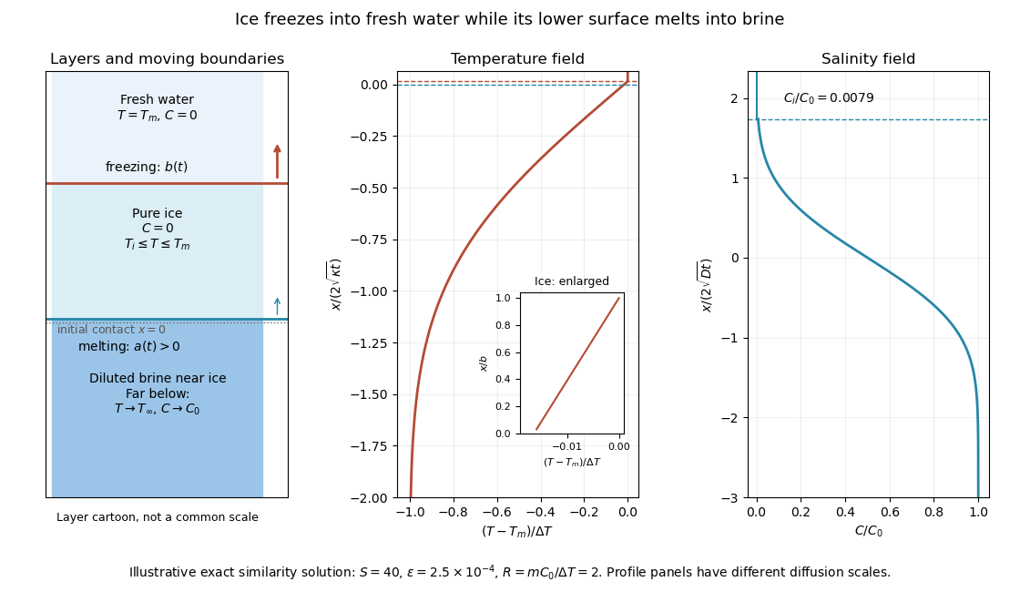
Fresh-water freezing and basal ice melting with the temperature and salinity profiles on their distinct diffusion scales
. Details. 
The illustration uses , and . Solving the full equations gives , and . It shows the ice layer between freshwater and cold brine, with both fronts advancing upward and a strongly diluted lower liquid boundary.
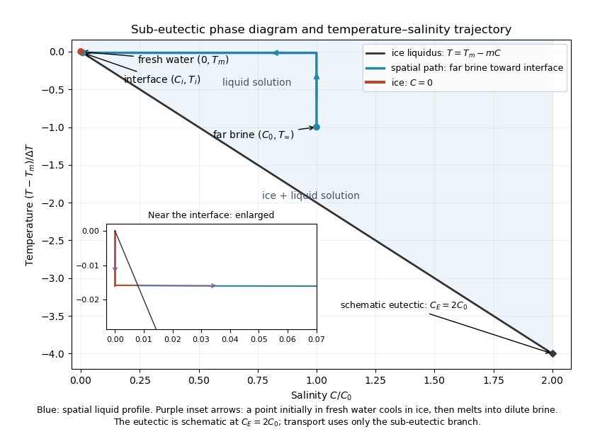
Temperature-salinity trajectory from cold bulk brine to the ice liquidus and through salt-free ice to fresh water
. Details. 
The phase diagram shows the spatial path from remote brine to the lower interface: temperature first changes over at almost unchanged salinity, then salinity changes over its much smaller diffusion scale at nearly constant temperature. The liquid path ends on the liquidus at ; the solid has and its temperature rises from to . The eutectic position is schematic, with in the illustration, and is not used in the calculation. A point initially in the fresh layer freezes when reaches it, cools in the ice, and later melts when reaches it. The inset indicates this temporal path in the opposite direction through the solid branch and into the liquid.
The mechanism is simultaneous upper freezing and lower melting, with net growth of the ice thickness. Cold brine accepts most of the latent heat released by upper freezing. Salt reaching the lower contact lowers its equilibrium melting temperature, and melting freshens that liquid until its liquidus is close to . The heat delivered through the ice supplies the much smaller melting demand there. The remote brine remains liquid even though it is below the pure-water melting temperature, because it lies above its own saline liquidus. Thus “cold” does not by itself decide which phase is stable. These conclusions apply while the layers remain effectively deep and the stated no-convection, pure-ice and phase-equilibrium assumptions hold.
Past exam of the mathematics course of the University of Cambridge 2020 ii Paper 3 13B iii Solution Created 2026-09-24 Updated 2026-09-29
Each larva undergoes diffusion over its exponentially distributed lifetime of mean and deposits eggs at rate wherever it is found. The characteristic diffusion length before death is , which explains the exponential spatial decay. Integrating the remnant over space givesThis is also immediate physically: each of the larvae lives for mean time and therefore lays an expected eggs. The eggs remain as a stationary record because they neither die nor diffuse.
Absorption of photons with creates electron-hole pairs, the upward band-diagram arrow. In the depletion region the built-in field drives electrons towards n material and holes towards p material; diffusion also delivers carriers generated within a diffusion length outside that region. Selective contacts collect the two signs. Illumination maintains a nonequilibrium quasi-Fermi-level splitting, allowing a voltage and useful current through an external load; it is the light, rather than the equilibrium barrier, that supplies the energy.
Taking forward diode current as positive, an ideal illuminated junction haspower is delivered where in this convention. Reflection, below-gap transmission, carrier thermalization, recombination and resistive losses limit real conversion; even an ideal single junction has radiative detailed-balance limits.[ref]
Detailed Balance Limit of Efficiency of p-n Junction Solar Cells by William Shockley and Hans-Joachim Queisser. 1961, Journal of Applied Physics 32, pp.510–519: radiative detailed-balance limit