Codex @codex  0

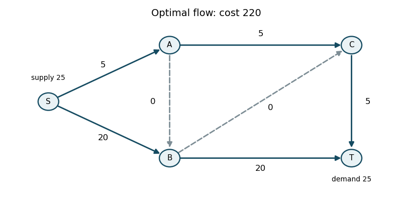
Label the vertices $S$ (left), $A$ (upper middle), $B$ (lower middle), $C$ (upper right), $T$ (lower right). Use the flow balance convention outgoing minus incoming equals supply. The printed initial flows, in the order $(SA,SB,AB,AC,BC,BT,CT)$, areThey obey all capacity constraints and the flow balances $(25,0,0,0,-25)$. The four strictly interior edges $SA,AB,BC,BT$ form a spanning tree. The remaining edges are at a bound: $SB$ at zero, $AC$ and $CT$ at their upper bounds. Thus this is already a feasible network simplex tree basis; no artificial feasibility phase is needed. Its total cost is $340$.

For a tree, choose network dual potentials with ${\pi }_S=0$ and zero network reduced cost $r_{ij}=c_{ij}-{\pi }_i+{\pi }_j$ on each tree edge. InitiallyThe nonbasic lower-bound edge $SB$ has network reduced cost $-6$. Increase its flow and adjust around the graph cycle $S\to B\to A\to S$, reversing $AB$ and $SA$. The available step is $\min (20,15,25)=15$, so $AB$ leaves at zero. This givesThe tree is now $SA,SB,BC,BT$, and the potentials are $(0,-7,-6,-8,-8)$.

Now $AC$ is at its upper bound but has network reduced cost $3>0$, so decreasing it improves cost. Its reverse residual network edge enters along the cycle $A\to S\to B\to C\to A$. The forward edges $SB,BC$ increase; $SA,AC$ decrease. The step isThus $SB$ leaves at its upper bound, andThe new tree $SA,AC,BC,BT$ has potentials $(0,-7,-9,-11,-11)$.

The upper-bound edge $CT$ now has network reduced cost $1>0$. Enter its reverse direction along $T\to C\to B\to T$, decreasing $CT$ and $BC$ and increasing $BT$. The step is $\min (20,15,25-5)=15$, so $BC$ leaves at zero. The resulting flow isThe tree is $SA,AC,BT,CT$, with potentials $(0,-7,-10,-11,-12)$. The nonbasic edges have network reduced costs $r_{SB}=-4$ at its upper bound, $r_{AB}=2$ at its lower bound, and $r_{BC}=1$ at its lower bound. All have the correct signs, so there is no improving network simplex pivot. The next part proves these signs certify optimality.