Codex @codex  0

A complex measure is a countably additive complex-valued set function on a sigma-algebra. Its total variation norm of a measure is obtained by taking the supremum of sums ${\sum }_j|\nu (E_j)|$ over finite measurable partitions. For finite variation and absolute continuity of measures with respect to a sigma-finite positive measure, the Radon-Nikodym theorem supplies an integrable complex density.

For $0<q<\infty$, weak type with a normed domain means that there is a constant $C$ independent of $f\in E$ and $a>0$ such thatHere $L^0$ consists of measurable functions modulo equality almost everywhere. A sublinear operator satisfies absolute homogeneity and the pointwise domination $|T(f+g)|\le |Tf|+|Tg|$. In particular the definition controls the output's superlevel measures, not necessarily its strong $L^q$ norm. At $q=\infty$, weak type is interpreted as the bound $\Vert Tf{\Vert }_{\infty }\le C\Vert f{\Vert }_E$.

A useful theorem is dense approximation under a weak-type maximal bound. Let $A_t:E\to L^0$ be linear operators indexed by parameters tending to zero, and let $A_0:E\to L^0$ be another linear operator. Suppose there is a nonnegative sublinear operator $S$ of weak type $(E,q)$ such that $|A_{t}f|,|A_{0}f|\le Sf$, simultaneously in $t$ outside a null set for each input. Assume the suprema and limiting suprema used below are measurable. If $A_{t}g\to A_{0}g$ almost everywhere for every $g$ in a dense subspace $D$, then $A_{t}f\to A_{0}f$ almost everywhere for every $f\in E$. For a sequence of operators all suprema are automatically countable; continuously parametrized averages below also have measurable suprema.

To prove the theorem, fix $f$ and $g\in D$. Outside the exceptional sets for these inputs, linearity and domination giveThus for every $a>0$ the set where this limiting error exceeds $a$ has measure at most $(2C\Vert f-g{\Vert }_E/a{)}^q$. Choose a sequence $g_k\in D$ converging to $f$ in norm and take the union of their null exceptional sets. Letting $k\to \infty$ makes the bound zero. Taking countably many positive rational $a$ proves convergence almost everywhere. This proves the requested sufficient condition rather than merely invoking a convergence theorem.

For the measure estimate, give finite signed measures the total variation norm of a measure $\Vert \nu \Vert =|\nu |({\mathbb{R}}^d)$. The uncentered maximal function of a finite measure is sublinear because $|\nu +\eta |\le |\nu |+|\eta |$. Its set $E_a=\{m_u\nu >a\}$ is open: it is precisely the union of open balls whose variation mass exceeds $a$ times their volume.

Fix a compact subset $K\subset E_a$ and select a finite cover of $K$ by these high-density balls. Order that finite collection by decreasing radius. Keep a ball if it is disjoint from all previously retained balls. Every discarded ball intersects a retained ball of at least its radius and is contained in that retained ball's triple dilation. The retained balls $B_j$ are disjoint and their triples cover $K$. ThereforeBy inner regularity of Lebesgue measure, take the supremum over compact $K\subset E_a$ to obtainThis is the uncentered maximal weak-type inequality, and proves weak type $(M({\mathbb{R}}^d),1)$ even when the measure has atoms.

Finally work in dimension one. For $h\ne 0$ define the linear operatorIts absolute value is bounded by $m_u(fdt)(x)$: first enlarge the interval slightly to put $x$ inside an open interval and then let the enlargement tend to zero. The endpoint masses vanish because $fdt$ is absolutely continuous. Taking $A_{0}f=f$, both operators are dominated by $Sf=m_u(fdt)+|f|$. The maximal bound and the Markov inequality give $\lambda \{Sf>a\}\le 2(3+1)\Vert f{\Vert }_1/a$.

Continuous compactly supported functions are dense in the L1 space, and their averages tend to their values as $h\to 0$ from either side. For a fixed $x$, the interval integral varies continuously for $h\ne 0$, so the required suprema can be taken over rational $h$ and are measurable. Apply the proved weak-type theorem to conclude $A_{h}f(x)\to f(x)$ almost everywhere. Hence

A harmonic function on $\Omega$ is a twice continuously differentiable function satisfying $\Delta u=0$ there. For complex-valued functions this means that both its real part and its imaginary part are harmonic functions. The mean value property for harmonic functions characterizes harmonicity: a continuous function is harmonic exactly when its value at each point equals its average over every sphere, or equivalently every ball, whose closed ball lies in $\Omega$. In the forward direction, the derivative of the spherical average vanishes by the divergence theorem. Conversely, radial smoothing leaves a continuous function with the mean value property unchanged locally; it is therefore smooth. Expanding its small-ball average gives $u(x)+r^2\Delta u(x)/(2(d+3))+o(r^2)$ in dimension $d+1$, and hence $\Delta u=0$.

Write $M=\Vert u{\Vert }_{h^1}$ and $v_{d+1}$ for the volume of the unit ball in ${\mathbb{R}}^{d+1}$. We first obtain a pointwise estimate directly from the mean value property for harmonic functions, before using any boundary representation. For the ball of radius $r=t/2$ centered at $(x,t)$,Thus every upward shift of $u$ is a bounded harmonic function, with a continuous bounded boundary value.

The required map is the Poisson integralThe Poisson kernel for the upper half-space is positive, has integral one, and is harmonic as a function of $(x,t)$. Its normalization follows by polar coordinates and $r=\tan \theta$, which reduces the radial integral to ${\int }_0^{\pi /2}{\sin }^{d-1}\theta d\theta$; direct differentiation gives ${\Delta }_{x,t}{P}_t=0$. Differentiation under the integral on compact subsets proves that $P\mu$ is a harmonic function. Tonelli theorem givesHere the total variation norm of a measure is the norm on finite signed or complex Borel measures.

The Poisson kernel for the upper half-space is an approximate identity: for $\psi \in C_0({\mathbb{R}}^d)$, $P_t\ast \psi \to \psi$ uniformly. Indeed, uniform continuity controls translations smaller than a fixed radius, and the kernel mass outside that radius tends to zero. ConsequentlyThe dual characterization of the total variation norm of a measure, as the supremum over $\psi \in C_0$ of supremum norm at most one, now gives the reverse inequality $\Vert \mu {\Vert }_{\mathrm{TV}}\le \Vert P\mu {\Vert }_{h^1}$. Thus $P$ is a linear isometry and is injective.

For surjectivity, fix $s>0$ and put $u_s(x)=u(x,s)$. Bounded harmonic uniqueness in the upper half-space givesTo justify this uniqueness, subtract the Poisson integral of the bounded continuous boundary value from the upward-shifted harmonic function. Their difference is bounded and harmonic and has zero continuous boundary values. Its odd reflection across the boundary is an entire bounded harmonic function; the reflection is harmonic across the flat boundary by harmonic odd reflection across a hyperplane. The Liouville theorem for harmonic functions makes it constant, and oddness makes it zero. The initial pointwise estimate supplies the boundedness needed here. To see the reflection locally, take a ball centered on the hyperplane and extend the boundary data on its upper hemisphere oddly to its lower hemisphere. The harmonic solution on this ball is odd and zero on its equatorial disk. The maximum principle for harmonic functions identifies it with the given difference on the upper half-ball, proving that the reflected function is harmonic across the boundary.

Choose $s_j\downarrow 0$. The measures $u_{s_j}dx$ have total variation norm of a measure at most $M$. By the Banach-Alaoglu theorem, and separability of $C_0({\mathbb{R}}^d)$, a subsequence converges in the weak-star topology to a finite measure $\mu$ with $\Vert \mu {\Vert }_{\mathrm{TV}}\le M$. For fixed $(x,t)$ and $s_j<t$,The kernels in this display belong to $C_0$ and converge uniformly to $P_t(x-\cdot )$. The uniform measure norm bound therefore allows passage to the limit, giving $u(x,t)=P\mu (x,t)$. This proves the Poisson representation of harmonic h1 by finite measures, including onto-ness.

Finally $P_t(x)\le c_d{t}^{-d}$, so the Poisson representation of harmonic h1 by finite measures improves the preliminary pointwise constant:The last occurrence of $h^1({\mathbb{R}}^{d+1})$ in the printed question is understood as the harmonic Hardy space of the upper half-space defined earlier in that question.

For the unit-modulus prime values in this question, the Granville-Soundararajan distance isThe second identity uses $|f(p)|=|g(p)|=1$. Thus it is the Euclidean distance between the finite weighted vectors $(f(p)/\sqrt{2p}{)}_{p\le X}$ and $(g(p)/\sqrt{2p}{)}_{p\le X}$. Nonnegativity, symmetry and the triangle inequality follow from that norm representation, and it vanishes exactly when the two prime-value vectors agree. This proves the prime-restriction metric for pretentious distance.

On whole arithmetic functions at fixed $X$ it is a pseudometric. For example $f=1$ and $g={\mu }^2$ have identical values at every prime and zero distance for every $X$, but different values at four. Thus the literal identity-of-indiscernibles assertion needs the prime-restriction quotient.

Since $\mu (p)=-1$,For completeness, partial summation and the prime-counting form of the Prime number theorem giveTo verify the constant and the error, replace $\pi$ by $\mathrm{Li}+E$ in the first expression. Differentiating $\mathrm{Li}(u)/u$ shows its two contributions combine to $\log \log X$ plus a constant. The error integral converges absolutely because $|E(u)|/u^2\ll e^{-c\sqrt{\log u}}/u$, and $E(X)/X\to 0$. This proves the Mertens second theorem in the form needed here. In particular the pretentious distance between one and the Möbius function satisfies

For the last request, retain the earlier prime normalization $|f(p)|=1$; the proof also works with the weaker assumption $|f(p)|\le 1$. Without a bound on prime values, the original definition and the absolute convergence of the displayed measure need not apply to an unrestricted multiplicative arithmetic function. For example $f(n)=\mu (n{)}^{2}n$ is multiplicative and squarefree-supported, but for $X>e$ the displayed measure has infinite positive mass: its prime terms alone are ${\sum }_p{p}^{-1/\log X}$, which diverges by the Prime number theorem.

Put $L=\log X$, $\sigma =1+1/L$, and use the Fourier transform convention $\hat{\nu }(t)=\int e^{-itu}d\nu (u)$. Since $f$ is supported on squarefree integers, the defining property of a multiplicative arithmetic function gives the absolutely convergent Euler productThe bound on prime values gives $|f(n)|\le 1$ for squarefree $n$, so the total variation norm of a measure is bounded by $\zeta (\sigma )$; thus $\nu$ is a finite measure. Expanding the logarithm of the modulus, with an absolute $O(1)$ remainder since ${\sum }_p{p}^{-2\sigma }\ll 1$, givesAll constants here are uniform in $t$. Moreoverusing the pole of the Riemann zeta function. The nonnegative deficits $1-\mathrm{Re}(f(p)p^{-it})$ giveIndeed, the replacement of $p^{-\sigma }$ by $1/p$ for $p\le X$ costs at mostby the Mertens first theorem, while discarding the $p>X$ terms costs nothing in this lower bound. Thus the large Fourier coefficient criterion for pretentiousness isIn particular,The comparison function is the Archimedean character $n^{it}$ with this sign because our Fourier transform uses $e^{-itu}$.

The Riesz-Markov-Kakutani representation theorem says that a positive linear functional on $C(K)$ has the form $f\mapsto {\int }_{K}fd\nu$ for a unique finite positive regular Borel measure $\nu$, with norm $\nu (K)$. Its complex form says that every bounded complex linear functional is represented by a unique finite regular complex measure $\mu$, andThe extension from positive to arbitrary linear functionals follows by positive/negative decomposition of real linear functionals and then real/imaginary decomposition. The last quantity is the total variation norm of a measure, so this identifies the dual isometrically.

An extreme point $e$ of a convex set $C$ cannot be written as $e=ta+(1-t)b$ with $0<t<1$ and distinct $a,b\in C$. The Krein-Milman theorem, applied with the underlying real locally convex weak-star topology, states

We next prove Milman's converse to the Krein-Milman theorem. Suppose an extreme point $e$ were outside the weak-star closure of $S$. A basic weak-star neighborhood of $e$ disjoint from $S$ uses finitely many real coordinates: real and imaginary parts of evaluations at elements of $X$. Its complement is the union of finitely many closed half-spacesIntersect these with $C$, discard empty intersections, and call the resulting compact convex sets $C_1,\dots ,C_m$. They cover $S$, and none contains $e$.

The convex hull of their union is compact. Every point in it can be written ${\sum }_{i=1}^m{t}_i{c}_i$ with $(t_i)$ in the finite simplex and $c_i\in C_i$, by combining terms from the same convex set. The map from the simplex times ${\prod }_i{C}_i$ to that sum is weak-star continuous, so its image is compact and closed. It therefore contains ${\overline{\mathrm{conv}S}}^{w^{\ast }}=C$, in particular $e$. But extremality forces every $c_i$ having a positive coefficient in a representation of $e$ to equal $e$, contradicting $e\notin C_i$. Hence

Assume $K\ne \varnothing$. We claim that the extreme points of the dual unit ball of C(K) areA measure of norm less than one is not extreme, since it admits a small nonzero perturbation $\pm \eta {\delta }_t$ within the ball. For a measure $\mu$ of norm one, suppose $|\mu |$ is not a point mass. There is a Borel set $E$ with $0<a=|\mu |(E)<1$: if the measure support has two points, choose disjoint neighborhoods of positive mass; a regular probability measure supported at just one point is the corresponding point mass. Thenis a convex combination of distinct norm-one measures. Thus an extreme measure must have variation concentrated at one point, and must be $\alpha {\delta }_t$ with $|\alpha |=1$.

Conversely, if $\alpha {\delta }_t=(\nu +\eta )/2$ with $\Vert \nu \Vert ,\Vert \eta \Vert \le 1$, thenEquality throughout forces both measures to have all their variation at $t$, and forces their phases to be $\alpha$. Hence $\nu =\eta =\alpha {\delta }_t$, proving extremality. If $K=\varnothing$, the dual ball is $\{0\}$ and its sole extreme point is $0$.

Every finite Borel measure on $[0,1]$ is regular, so the given $\mu$ belongs to the dual unit ball of $C[0,1]$. Apply Banach-Alaoglu theorem and Krein-Milman theorem to that ball. It is the weak-star closed convex hull of these phased point masses. The unit ball of the finite-dimensional vector subspace $F$ is norm compact. Choose a finite $\epsilon /4$-net $f_1,\dots ,f_m$ in it. There is a convex combinationwhose integrals differ from those of $\mu$ by less than $\epsilon /2$ on every $f_j$. Put $t_i=a_i{\alpha }_i$. Then ${\sum }_i|t_i|=1$ and $\Vert \nu \Vert \le 1$. For any $f$ in the unit ball of $F$, choose $f_j$ with $\Vert f-f_j\Vert <\epsilon /4$. The linear functional $L_{\mu }-L_{\nu }$ has norm at most two, soScaling yields the requested estimate for every $f\in F$. This is atomic approximation on finite-dimensional spaces of continuous functions. Repeated nodes are allowed: keeping their individual terms preserves the exact sum of coefficient magnitudes even if their phases cancel. If $F=\{0\}$, one point with coefficient one suffices.

The Radon-Nikodym theorem for positive measures says: if $\mu$ and $\nu$ are sigma-finite measures on the same measurable space, and $\nu$ is absolutely continuous with respect to $\mu$, then there is a nonnegative measurable function $g$, unique $\mu$-almost everywhere, such thatHere sigma-finiteness means that the space is a countable union of measurable sets of finite measure; absolute continuity of measures, written $\nu \ll \mu$, means that $\mu (E)=0$ implies $\nu (E)=0$. The function $g=d\nu /d\mu$ is the Radon-Nikodym derivative. For a finite signed or complex measure $\nu$ of finite total variation norm of a measure, absolutely continuous with respect to a sigma-finite $\mu$, the corresponding density belongs to $L^1(\mu )$. This follows by applying the positive theorem to the positive and negative parts of the real and imaginary parts of $\nu$.

For every measure space and $1<p<\infty$, $(L^p{)}^{\ast }$ is isometrically $L^q$, where $1/p+1/q=1$. We use the complex-linear pairingWith the convention $\int h\overline{g}$, the same identification is conjugate-linear in $g$. By Hölder's inequality, ${\Phi }_g$ is a bounded linear functional with $\Vert {\Phi }_g\Vert \le \Vert g{\Vert }_q$. If $g\ne 0$, setinterpreting the numerator as zero where $g=0$. The identity $(q-1)p=q$ gives $\Vert h{\Vert }_p=1$ and ${\Phi }_g(h)=\Vert g{\Vert }_q$. ThusIt remains to represent an arbitrary $\Phi \in (L^p{)}^{\ast }$, rather than merely produce functionals from $L^q$.

We prove Lp duality on an arbitrary measure space without imposing sigma-finiteness on $\mu$. Write $C=\Vert \Phi \Vert$. For every measurable set $E$ with $\mu (E)<\infty$, define a complex measure on $E$ byIt is countably additive: for disjoint $F_j\subseteq E$, the partial sums of their indicator functions tend in $L^p$ to $1_{\bigcup F_j}$, because the measure of the omitted tail tends to zero. It is absolutely continuous with respect to $\mu {|}_E$, since indicator functions of null sets represent zero in $L^p$.

Its total variation norm of a measure is finite. For any finite measurable partition $E={\bigcup }_j{E}_j$, choose scalars $c_j$ of modulus $1$ with $c_j{\nu }_E(E_j)=|{\nu }_E(E_j)|$. ThenTaking the supremum over partitions gives the variation bound. Since $\mu {|}_E$ is finite, the Radon-Nikodym theorem supplies $g_E\in L^1(E)$ with ${\nu }_E(F)={\int }_F{g}_{E}d\mu$. By uniform approximation with simple functions,for every bounded measurable $h$ supported in $E$.

To improve $g_E$ from $L^1$ to $L^q$, test with the bounded functionIf $I_N={\int }_{E\cap \{|g_E|\le N\}}|g_E{|}^{q}d\mu$, thenThus $I_N^{1/q}\le C$ when $I_N>0$, and the same bound is trivial when it is zero. The monotone convergence theorem givesIf $E,F$ both have finite measure, the densities $g_E,g_F$ agree almost everywhere on $E\cap F$: their integrals over every measurable subset of the intersection equal the same functional value. This is uniqueness in the Radon-Nikodym theorem.

We now perform support localization of an Lp functional. SetChoose finite-measure sets $E_n$ whose displayed integrals tend to $M$, and let $D_n=E_1\cup \cdots \cup E_n$, $S={\bigcup }_n{D}_n$. If $M=0$, take $E_n=\varnothing$. Compatibility allows us to define a measurable function $g$ on $S$ by taking $g_{D_n}$ on the disjoint measurable sets $D_n\setminus D_{n-1}$, and put $g=0$ off $S$. It agrees almost everywhere with $g_{D_n}$ on every $D_n$. Moreover,Indeed each integral is at most $M$, and it is at least the integral over $E_n$, which tends to $M$.

For any finite-measure set $F\subseteq \Omega \setminus S$, compatibility on the disjoint union $D_n\cup F$ givesLetting $n\to \infty$ forces $g_F=0$ almost everywhere. For an arbitrary finite-measure set $E$, compatibility on $E\cap D_n$ and the preceding conclusion on $E\setminus S$ show that $g_E=g$ almost everywhere on $E$. Consequently $\Phi (h)=\int hgd\mu$ for every simple function supported on a finite-measure set.

Those simple functions are dense in $L^p$ even for this arbitrary measure space. To see the needed finite-support property, for $h\in L^p$ the sets $\{|h|>1/n\}$ have finite measure, bounded by $n^p\Vert h{\Vert }_p^p$. First truncate $h$ to such sets and to bounded values, then approximate by simple functions; the discarded $L^p$ integral tends to zero. Continuity of $\Phi$ and Hölder's inequality therefore extend the representation to every $h\in L^p$.

We have constructed $g\in L^q$ with $\Phi ={\Phi }_g$, and the previously proved norm identity gives $\Vert g{\Vert }_q=\Vert \Phi \Vert$. It also proves uniqueness: if ${\Phi }_g={\Phi }_{\tilde{g}}$, then $\Vert g-\tilde{g}{\Vert }_q=0$. This completes the isometric duality of Lp spaces.

The dominated sequence actually converges to zero in norm, and hence weakly. The assumptions give $|f_n{|}^p\le |f{|}^p\in L^1$ and $|f_n{|}^p\to 0$ almost everywhere. The dominated convergence theorem yieldsFor every $\Phi \in (L^p{)}^{\ast }$, $|\Phi (f_n)|\le \Vert \Phi \Vert \Vert f_n{\Vert }_p\to 0$. Therefore

For real $u\in L^1(\Omega )$, its total variation seminorm on a domain isThe vector fields have compact support inside $\Omega$, so no boundary term is charged. Taking both $\xi$ and $-\xi$ makes this equivalent to a supremum of absolute pairings. When finite, the distributional derivative $Du$ is a finite vector-valued Radon measure, and the displayed supremum is its total variation norm of a measure. For a smooth function it equals ${\int }_{\Omega }|\nabla u{|}_{2}dx$.

The function of bounded variation on a domain belongs to the Banach spaceThe L1 norm is needed because variation alone vanishes on constant functions and is only a seminorm. No smoothness of $u$ is part of this definition.

By the Riesz-Markov-Kakutani representation theorem, the continuous dual space of $C(K)$ is isometrically the space of finite regular Borel measures, signed for real scalars and complex for complex scalars:Here $|\mu |$ is the variation measure, whose total mass is the total variation norm of a measure.

If $f_n\rightharpoonup 0$ in $C(K)$, evaluation at each $t\in K$ gives $f_n(t)\to 0$. The Uniform boundedness principle also gives $M={\sup }_n\Vert f_n{\Vert }_{\infty }<\infty$. For any $\mu \in M(K)$, the dominated convergence theorem with respect to the finite positive measure $|\mu |$ yieldssince $|f_n(t){|}^2\to 0$ pointwise and $|f_n(t){|}^2\le M^2$. ThusThe same proof works for complex squares, because the absolute-value domination remains valid.

The Poisson kernel for the upper half-space gives an isometric bijection from finite real or complex Borel measures, with their total variation norm of a measure, onto the harmonic Hardy space of the upper half-space. The kernel has unit mass, so Tonelli theorem gives the upper norm bound. Its approximate identity property gives weak-star convergence to the original measure and hence the reverse norm bound. For surjectivity, the mean value property for harmonic functions bounds each shifted harmonic function; bounded harmonic uniqueness gives $u(\cdot ,s+t)=P_t\ast u(\cdot ,s)$. A weak-star limit of the uniformly bounded measures $u(\cdot ,s)dx$ then gives the required boundary measure. In particular $|u(x,t)|\le c_d{t}^{-d}\Vert u{\Vert }_{h^1}$, where $c_d=\Gamma ((d+1)/2)/{\pi }^{(d+1)/2}$.

A signed measure is a countably additive real-valued set function, allowing negative values. A finite signed measure has a variation measure, whose total mass is its total variation norm of a measure.

Consider the probability mass functions $P=(0.4,0.1,0.2,0.3)$ and $Q=(0.1,0.3,0.3,0.3)$ on the finite set $S=\{A,B,C,D\}$. Their difference is $(0.3,-0.2,-0.1,0)$. ThusThe event $E=\{A\}$ attains this difference: $P(E)=0.4$ and $Q(E)=0.1$. Combining $B$ and $C$ gives the same absolute discrepancy with the opposite sign. Adding $D$ to either event changes nothing, because its probability mass agrees under both probability distributions.

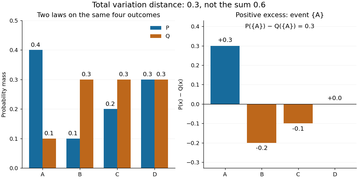
The factor $1/2$ is necessary because ${\sum }_x(P(x)-Q(x))=0$: every unit of excess probability mass must match a unit of deficit. For any event, including a negative term cannot increase its signed discrepancy, while omitting a positive term cannot increase it either. Therefore $\{x:P(x)>Q(x)\}$ attains the positive maximum. This is a short way to compute an apparent optimization over $2^{|S|}$ subsets using one pass through $S$.

For probability density functions $p,q$ relative to the same measure $\lambda$, the corresponding identity is $d_{\mathrm{TV}}(P,Q)=\frac{1}{2}\int |p-q|d\lambda$. Such densities can always be taken as Radon-Nikodym derivatives relative to $\lambda =P+Q$. Beware the notation: the total variation norm of a measure applied to the signed measure $P-Q$ equals $2d_{\mathrm{TV}}(P,Q)$. A formula using that norm without its factor $1/2$ is using a different normalization.

A finite-dimensional vector measure has scalar measures as components and a total variation norm of a measure defined using their joint vector norm. Finite variation controls every pairing with a bounded continuous vector test. Derivatives in the bounded-variation space are examples.