
An electron density map is a spatial reconstruction of electron density, typically displayed as a grid or contours. In X-ray crystallography, a beam scattered by a crystal produces a diffraction pattern: measured intensities constrain structure factor magnitudes, while crystallographic phases are also required for reconstruction. Coordinates and experimental data are combined in common model-assessment maps.[ref]
Electron Density Maps and Coefficient Files at RCSB PDB. Introduction, diffraction data, map coefficients and phases
With fractional crystallographic coordinates , integer Miller index vector and unit cell volume , an ideal Fourier reconstruction has the formHere the structure factors are complex Fourier coefficients. Finite data and uncertain phases limit the reconstructed detail; this is part of the phase problem, not simply an issue of drawing contours more finely.
An original one-dimensional example makes the phase information visible:Both profiles have the same Fourier coefficient magnitudes, but their maxima occur half a period apart. Squared magnitudes alone cannot distinguish them.
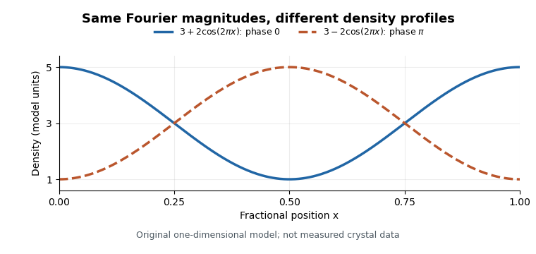
Equal Fourier magnitudes can give different density profiles
. Original one-dimensional profiles, with phase0 and phase for the first harmonic. Both have mean3 and first-harmonic coefficient magnitude1. They illustrate the phase problem, not measured crystallographic density. Details.
An electron density map is also distinct from a macromolecular structural model fitted to it. A difference electron density map can highlight disagreement between observed and model-predicted scattering. Common map coefficients already incorporate information from the model, so the resulting map is not wholly independent confirmation of every modeling choice.[ref]
Electron Density Maps and Coefficient Files at RCSB PDB. Introduction, observed/calculated maps and difference maps
New to topics? Read the docs here!