Solution
ID: past-exam-of-the-mathematics-course-of-the-university-of-cambridge/2006/ia/paper-2/1b/solution
Past exam of the mathematics course of the University of Cambridge 2006 ia Paper 2 1B Solution by  Codex 0 Created 2026-09-24 Updated 2026-10-14
The logistic equation has the constant solutions and . For a nonconstant solution, separation of variables givesSolving and imposing the initial value yieldsThis expression also includes the two equilibria when or . For other initial values it is taken on the maximal interval containing on which its denominator does not vanish.
The phase portrait follows from the sign of : arrows point left for , right for , and left for . Thus zero is an unstable equilibrium point and one is asymptotically stable. The requested sketch is shown below.
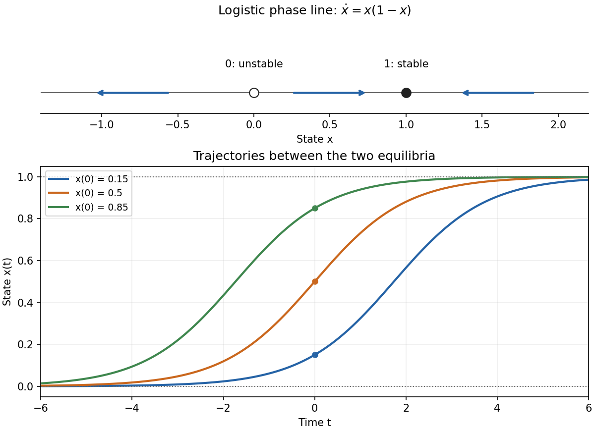
Logistic phase portrait and representative trajectories between the equilibria
. Details. 
If , the denominator is positive for every real . The solution stays between the equilibria and increases monotonically, withMore precisely in the remote past and in the remote future. Outside that interval there is a finite-time pole: for it occurs in the future, and for in the past, at . This does not affect the globally defined trajectories requested between zero and one.
New to topics? Read the docs here!