 Solution

import numpy as np
import matplotlib.pyplot as plt

def hill(u, K, n):
    u = np.asarray(u)
    return u**n / (K**n + u**n)

X_grid = np.linspace(0, 5, 501)
Y_eq = 2 * hill(X_grid, 1, 2)
Z_eq = 3 * hill(X_grid, 2, 4)
plt.figure(figsize=(6, 4))
plt.plot(X_grid, Y_eq, label="Y equilibrium: K=1, n=2")
plt.plot(X_grid, Z_eq, label="Z equilibrium: K=2, n=4")
plt.xlabel("X concentration")
plt.ylabel("Equilibrium concentration")
plt.legend()
plt.tight_layout()
plt.show()

The Hill constant sets the half-maximum input:

Y^{*} (1) = 1

and

Z_{direct}^{*} (2) = 1.5

. Increasing that constant shifts activation toward larger

X

. The Hill coefficient changes steepness rather than the half-maximum position; the normalized slope at

X = K

n / (4 K)

. Because the two examples also differ in

K

and maximal production, compare normalized responses when isolating the effect of

n

alone. Both curves vanish at zero and saturate toward their respective maxima.

Figure 1.
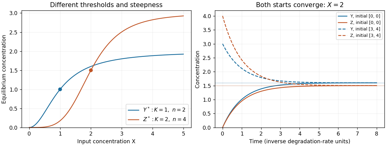
Independent Hill activation and convergence from two initial states
. The left panel shows different half-activation inputs and Hill coefficients. The right panel integrates the two independent output equations at fixed X=2; dashed curves start above equilibrium and solid curves start at zero. **Details**.

 Read the full article

 New to topics? Read the docs here!