Codex @codex 0
Joined 2026-09-21 Message

Incoming links: Capacitor energy
For an isolated smooth conducting sphere of radius , Gauss's law gives surface electric field . Combining its capacitance with capacitor energy gives the displayed bound when the surrounding medium has dielectric strength and approximately vacuum permittivity. Nearby conductors, surface roughness and discharge geometry can lower the practical limit.
Capacitance Created 2026-09-24 Updated 2026-10-18
The capacitance of a linear two-terminal capacitor is the constant relating its separated electric charge to its terminal electric potential difference:Here is the electric charge on one electrical conductor, the other carries , and is their electric potential difference with the same ordering. Reversing the terminal ordering reverses both and and leaves capacitance unchanged. An ideal passive capacitor has ; an ordinary pair of separated electrical conductors with positive permittivity has . At , use rather than the undefined ratio .
For example, electric charge magnitude at terminal electric potential difference gives capacitance . At , the same linear capacitor has and the same capacitance. The plots in capacitor energy show that capacitance is the slope of the electric charge versus terminal electric potential difference graph.
For fixed geometry and linear material response, capacitance depends on dimensions and permittivity, rather than the source's terminal electric potential difference. This is why capacitance is a useful property of a component: once it is known, predicts the separated electric charge for each operating terminal electric potential difference. The SI unit is the farad, . [ref].
For combinations of capacitors, the same terminal definition gives an equivalent capacitance. Two identical capacitors of capacitance connected in parallel share the same terminal electric potential difference, and their electric charges add, giving . Connected in series with an initially neutral isolated junction, they carry equal plate electric charge magnitudes and their terminal electric potential differences add, giving . [ref].
Capacitor Created 2026-10-03 Updated 2026-10-13
A capacitor stores electrostatic energy by separating electric charge between two electrical conductors. In the ideal two-terminal model their electric charges are and , with a vacuum or insulating gap preventing direct transfer between them. Write for the terminal electric potential difference, where and are the electric potentials of the two electrical conductors. A linear capacitor obeyswhere its capacitance depends on the geometry and permittivity, and is independent of the applied electric potential difference while these stay fixed. [ref].
For example, the parallel-plate capacitor below has capacitance . At terminal electric potential difference , the electric charge magnitude on either plate isThe total electric charge of the device is : charge neutrality does not imply zero capacitor energy. This capacitor stores in its electric field. The schematic in parallel-plate capacitor shows the separation of electric charge; the plots in capacitor energy show how storage grows with terminal electric potential difference.
The useful distinction is between storing net electric charge and storing separated electric charge. A capacitor can release electrostatic energy into an electrical circuit; in an ideal RLC circuit, energy moves between the capacitor's electric field and the magnetic field associated with inductance. An ideal disconnected capacitor retains its separated electric charges and capacitor energy because there is no path for discharge.
Capacitor energy Created 2026-10-03 Updated 2026-10-14
The capacitor energy is the electrostatic energy stored when electric charge is separated. For a linear capacitor of fixed positive capacitance , plate electric charge magnitude , and terminal electric potential difference , it isThe zero is the uncharged state. Thus the capacitor energy is positive for nonzero , even though the total electric charge of the two plates is zero. [ref].
For the parallel-plate capacitor example, capacitance and terminal electric potential difference giveThe plate electric charge magnitude is . Doubling terminal electric potential difference with capacitance unchanged doubles the plate electric charge magnitude and quadruples the capacitor energy.
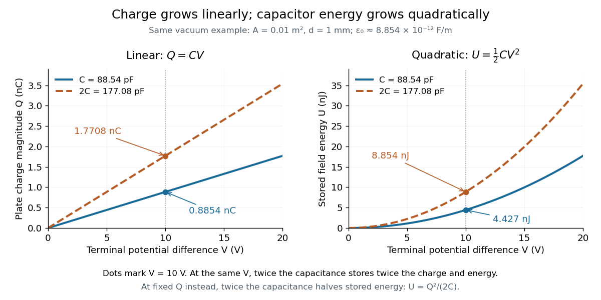
The electric charge is a linear function of terminal electric potential difference, while capacitor energy is a quadratic function. The second curve in each plot uses twice the capacitance: at a given terminal electric potential difference, both plate electric charge magnitude and capacitor energy double. These relations let us calculate how much energy an electrical circuit can receive when a capacitor discharges.
A brief charging argument explains the factor . If the plate electric charge magnitude has reached , the terminal electric potential difference is . Transferring a further amount of electric charge quasistatically requires work . With the geometry and permittivity fixed, the integral isUsing gives the other two forms. This integral accounts for the gradually rising terminal electric potential difference; it is the work stored in the capacitor's electric field, rather than a claim that all energy drawn from a fixed-voltage battery during charging ends up stored.
The field picture gives the same result. In the vacuum gap of a parallel-plate capacitor, the electric field has energy density . Multiplying by the gap volume gives the electrostatic energyFor the worked example, and reproduce . The electrostatic energy resides in the electric field throughout the gap, despite overall charge neutrality.
When capacitance changes, specify the constraint. At fixed plate electric charge magnitude , increasing capacitance decreases capacitor energy ; doubling capacitance halves it. At fixed terminal electric potential difference , increasing capacitance increases capacitor energy ; doubling capacitance doubles it. In the latter case a connected battery supplies additional electric charge and energy, and there may also be mechanical work. Use the fixed-voltage capacitor energy balance to account for all transfers before inferring a force from changing capacitor energy.
Dielectric Created 2026-10-14 Updated 2026-10-18
A dielectric is a material in which an electric field produces electric polarization while transport of electric charge is sufficiently small for the intended use. An insulating solid in a capacitor is an example; real dielectrics can still have dielectric loss and nonzero electrical conductivity.
The important distinction is between rearranging bound electric charge and transporting mobile charge carriers through the specimen. Bound electric charges can move a little within a chemical atom or molecule, or an existing electric dipole can turn. Their averaged electric dipole moments produce electric polarization even if there is negligible steady electric current between the electrodes. A changing electric polarization does give a bound current; the absence of steady conduction does not mean that the material is electrically unresponsive.[ref]
For uniform electric polarization in a rectangular slab, polarization density gives zero bound volume charge density in the interior and opposite bound surface charge densities on the left and right faces. The electric charge has been redistributed, not created. More generally, the divergence theorem makes the cancellation explicit:Here is the outward normal vector on the material boundary. This accounts for both bound volume charge density and bound surface charge density; omitting either can falsely suggest that an initially neutral dielectric acquired net electric charge.
An electrical insulator between capacitor plates supports a useful combination: appreciable electric polarization, little leakage electric current, and tolerance of the intended electric field. This lets a small parallel-plate capacitor store separated electric charge and recoverable capacitor energy. The comparison in dielectric capacitor response explains why specifying fixed electric charge or fixed electric potential difference changes the answer. High relative permittivity alone does not establish good insulation or a large usable energy density; dielectric loss and dielectric breakdown matter as well.
Dielectric capacitor response 2026-10-14
Compare two initially identical parallel-plate capacitors with plate area , fixed gap , vacuum capacitance , and initial electric potential difference . Completely fill both gaps with the same uniform linear dielectric of static relative permittivity , neglecting the fringing field of a capacitor. Keep one connected to an ideal voltage source and isolate the other. The geometric capacitance becomes in both cases; the electrical constraint determines what else changes.[ref]
8.4 Capacitor with a Dielectric. §8.4, Figure 8.17 and equation (8.11): isolated capacitor, unchanged free plate charge and increased capacitance
Write , and . Applying , and the capacitor energy formula gives the complete comparison:Thus the statement that a dielectric reduces the electric field needs the fixed-free-charge condition. With fixed electric potential difference, the voltage source supplies additional free plate electric charge, maintaining despite the new bound electric charges.
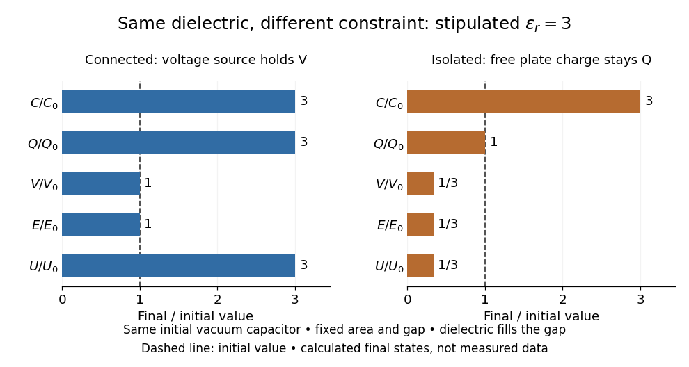
Dielectric capacitor response at fixed voltage and fixed charge
. Original normalized comparison for the stipulated model : every ratio is relative to the same initially charged vacuum capacitor. The dashed line marks the initial value. The bars show final values, not a time history or measured data. Plate geometry is unchanged and the dielectric completely fills the gap. Details.For the stipulated example, the voltage source supplies . At constant , its delivered electrical work is , whereas the increase in capacitor energy is . In an ideal reversible quasistatic insertion, the remaining is mechanical work delivered by the assembly, as accounted for in fixed-voltage capacitor energy balance. For the isolated assembly, capacitor energy falls from to , allowing of mechanical work in the same ideal limit. Actual losses reduce recoverable work; energy increases in the connected case do not arise from the dielectric supplying free energy.
Dielectric strength Created 2026-10-14 Updated 2026-10-20
Dielectric strength characterizes the electric field at dielectric breakdown under specified test conditions. In an ideal uniform gap, it sets a voltage scale .[ref]
8.5 Molecular Model of a Dielectric. §8.5: dielectric strength definition and voltage limit for a specified plate separation
The parallel-plate capacitor model consequently gives the stored energy density scaleThis is a model scale, not an operating rating: fringing field of a capacitor make local electric fields differ from , while leakage and dielectric loss spend some supplied energy as heat. Comparing usable capacitor energy therefore requires insulation and breakdown performance as well as permittivity. Electrical reactance Created 2026-10-14 Updated 2026-10-20
Electrical reactance is the signed imaginary part of electrical impedance , measured in ohms. It describes the part of the terminal electric potential difference in phase quadrature with the electric current in a sinusoidal steady state. In the convention, an ideal inductor has and an ideal capacitor has for . A large reduces electric current at fixed applied voltage, but an ideal purely reactive component returns the energy it receives over each cycle. This is why electrical reactance and electrical resistance have the same units yet describe different physical behavior. [ref]
https://www.feynmanlectures.caltech.edu/II_22.html#Ch22-S5. Feynman, Leighton and Sands, The Feynman Lectures on Physics, II.22.5: resistance, reactance and energy loss
.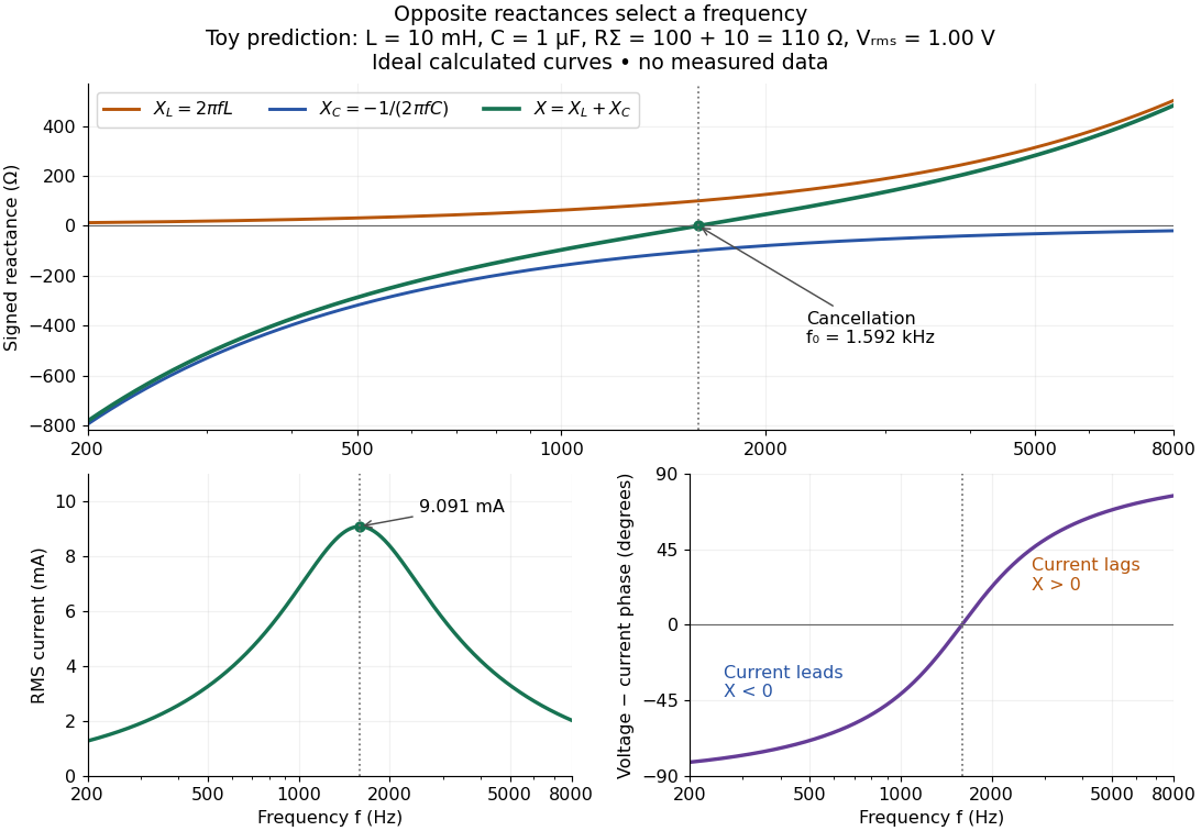
In a series RLC circuit, electrical impedances add because the same electric current passes through every component. For ideal positive inductance , capacitance , and total electrical resistance ,Here is voltage wave phase minus current wave phase. Below , and electric current leads terminal voltage; above it, and electric current lags. At , the two signed electrical reactances cancel, leaving and the maximum electric current at fixed terminal voltage. This is the resonant series RLC response. Electrical resistance does not cancel: the toy circuit gives and there. These numbers follow directly from the stipulated component values. [ref]
University Physics Volume 2 by Samuel J. Ling and others. Ling, Moebs and Sanny, University Physics 2, §15.3: series impedance and resonance
.Cancellation concerns terminal voltage, not the disappearance of stored energy. In the toy circuit at resonance, the individual inductor and capacitor voltages are each in root mean square magnitude, with opposite wave phases, while their sum is zero. Their peak stored magnetic energy and capacitor energy are each , attained at different times. With smaller positive , either component voltage can exceed the applied voltage. This ability to select a frequency while sustaining internal energy exchange connects electrical reactance to tuning and frequency response.
For an ideal inductor or capacitor, the absorbed instantaneous power equals the rate of change of stored energy:Positive power stores energy; negative power returns it. Over a periodic steady state, each stored energy returns to its initial value, so its cycle-averaged absorbed power is zero. An ideal resistor instead has , transferring energy into Joule heating. More generally, the average terminal power of this series RLC circuit isZero average power in an ideal reactive component does not imply zero instantaneous power, zero electric current, or zero stored energy. Real coils and capacitors have losses, so zero ideal reactive loss is a model assumption rather than a claim about every component. [ref]
University Physics Volume 2 by Samuel J. Ling and others. Ling, Moebs and Sanny, University Physics 2, §15.4: instantaneous and average AC power
. Electric battery Created 2026-10-14 Updated 2026-10-20
An electric battery converts the available chemical Gibbs free energy of one or more galvanic cells into electrical work delivered to an electrical load. The reacting materials are a finite reservoir: a battery can sustain a terminal electric potential difference while discharging, but cannot supply energy indefinitely. Unlike a capacitor, whose capacitor energy resides in an electric field, a battery chiefly stores its available energy in the chemical state of its materials. The detailed half-reactions and apparatus of a Daniell cell explain this conversion at the electrode level.
During discharge, electrons move through metallic wires from the negative anode, through the electrical load, to the positive cathode; external conventional current points the other way. Inside the battery, ions carry electric current through the electrolyte, and redox chemical reactions connect ionic transport to electronic transport at the electrodes. The same electron does not make a lap through both wire and electrolyte. Electric charge conservation closes the circuit; changing chemical composition supplies the energy. See galvanic cell for the two transport paths and electrolyte for how oppositely moving ions contribute to one net electric current.
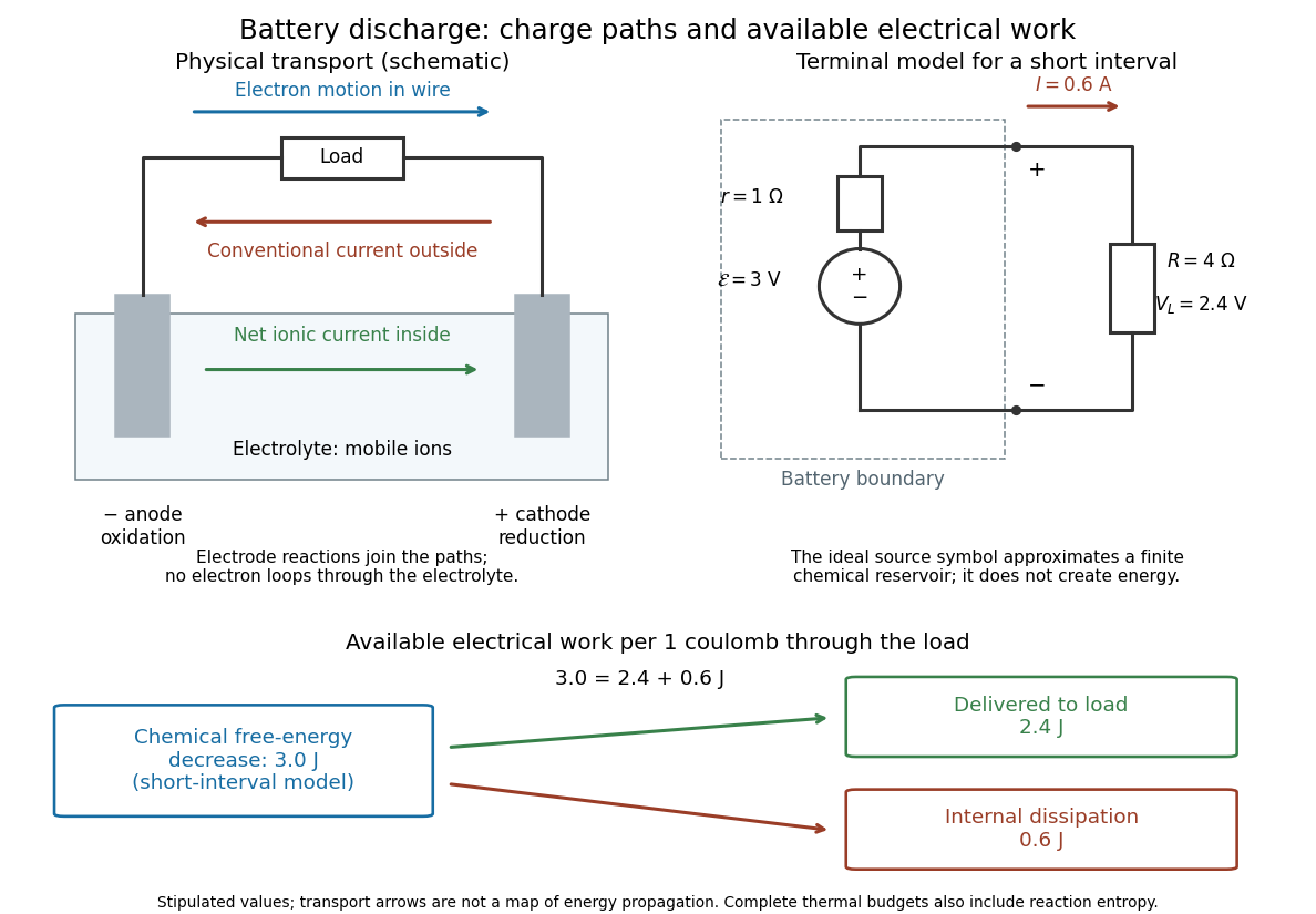
The source's electromotive force measures its driving work per unit electric charge, in volts; the loaded terminal electric potential difference measures the electrical work per unit electric charge delivered outside the battery. They agree in an ideal lossless source, or approximately near open circuit, but generally differ during discharge.[ref]
University Physics Volume 2 by Samuel J. Ling and others. §10.1, Introduction to Electromotive Force, work per charge and terminal voltage
In the ideal fixed-voltage model used in fixed-voltage capacitor energy balance, a battery maintains a prescribed terminal electric potential difference while electric charge flows to or from the capacitor. This is a constraint for that calculation, not an inexhaustible reservoir. The fixed-voltage capacitor energy balance also accounts for electrical energy returned to the source; an actual cell can accept sustained charging only if its chemistry and operating conditions permit it.
Fixed-voltage capacitor energy balance Created 2026-10-07 Updated 2026-10-20
For a quasistatic change of capacitance at fixed terminal electric potential difference, the capacitor energy is and plate electric charge is . Electrical work supplied to the electric field by the battery is , so mechanical work done on the capacitor is . Increasing the separation of a parallel-plate capacitor makes : mechanical work is positive even though electrostatic energy decreases, because electrical energy returns to the source. Conversely, when , the battery supplies : half increases capacitor energy and half is available as mechanical work done by the electric field. Differentiating capacitor energy alone at fixed terminal electric potential difference omits this exchange with the battery.
Inductance Created 2026-09-24 Updated 2026-10-13
Inductance relates electric currents to the magnetic flux linkage they produce. For a single linear coil with fixed geometry and magnetic response, its self-inductance is the constant inHere is magnetic flux linkage from the coil's own electric current . The SI unit of inductance is the henry. Knowing inductance lets us predict the induced electromotive force when electric current changes, and the magnetic energy stored by an inductor. [ref].
For example, a coil of self-inductance carrying electric current has magnetic flux linkage . If its turns link the same magnetic flux, each turn has magnetic flux . Keeping the geometry and magnetic response fixed while doubling electric current doubles magnetic flux linkage and quadruples the inductor's magnetic energy.
The comparison with capacitance is useful: a linear capacitor has and stores capacitor energy in its electric field, whereas a linear inductor has and stores magnetic energy in its magnetic field. The RLC circuit brings both forms of energy storage together.
Parallel-plate capacitor Created 2026-10-14 Updated 2026-10-18
A parallel-plate capacitor consists of two parallel electrical conductors with overlapping area and separation . If the gap is small compared with both plate widths and is filled by a uniform material of positive permittivity , its capacitance is approximatelyThis neglects the fringing field of a capacitor near the plate edges. The interior electric field points from the plate of positive electric charge to the plate of negative electric charge, and is approximately uniform. [ref].
For a worked vacuum example, stipulate , , and vacuum permittivity . This rounds the value in Fundamental Physical Constants — Complete Listing by National Institute of Standards and Technology and others. Within the approximation,At terminal electric potential difference , the electric field magnitude is , the plate electric charge magnitude is , and the capacitor energy is . These numbers use the stipulated rounded vacuum permittivity; finite plates also have corrections from the fringing field of a capacitor.
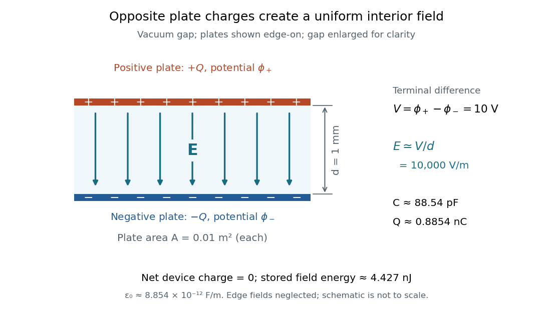


The formula makes design changes easy to predict: doubling the overlapping area doubles the capacitance, and halving the gap doubles the capacitance, with permittivity fixed and the fringing field of a capacitor neglected. Doubling permittivity also doubles capacitance if the material uniformly fills the gap and remains linear. This lets a compact device store more separated electric charge at the same terminal electric potential difference.
The short derivation uses surface charge density . In the interior, Gauss's law gives electric field magnitude . The electric potential difference is , so dividing by gives . A narrow curved capacitor gap has the same leading local approximation when its width is much less than the curvature radius.
Past exam of the mathematics course of the University of Cambridge 2013 ib Paper 4 7D Solution Created 2026-09-24 Updated 2026-10-07
The grounded conducting plane supplies the induced charge needed for a uniform field between the plates and zero field above the upper plate. Gauss's law gives in the gap. With electric potential zero at the grounded plate,Integrating the electrostatic energy density across the gap gives the capacitor energy per unit areaFor an isolated upper plate, charge is fixed, so increasing to gives exactly , with its initial value. The positive increase equals the mechanical work done against attraction.
At fixed voltage, the new charge density is , and the energy becomes . Consequently . Charge per unit area flows back to the voltage source, which receives energy . The externally supplied mechanical work is still : the field loses half this returned electrical energy and the mechanical work supplies the other half. Thus the fixed-voltage capacitor energy balance includes both field and source energy.
Past exam of the mathematics course of the University of Cambridge 2018 ib Paper 3 17C Solution Created 2026-09-24 Updated 2026-10-03
Take the dot product of Ampère-Maxwell equation with and of Faraday's law with . The divergence of a cross product identitythen gives the local Poynting theoremIntegration and the divergence theorem produce the stated equation. Its terms are the rate of change of electromagnetic energy, the work per unit time done on charges, and the outward flux of the Poynting vector .
Let the plate separation be and their radius be , so . Between the plates,For a circular Amperian loop of radius , the displacement current in the Ampère-Maxwell equation givesThereforewhich points radially outward. Its flux through the cylindrical side is , exactly for the stored capacitor energy .
Past exam of the physics B course of the University of Cambridge 2015 Paper 1 Section A A1 Solution 2026-10-20
For a smooth isolated conducting sphere, Gauss's law gives the surface electric field and electric potential . At the specified dielectric strength, . The capacitance of an isolated conducting sphere is , so its capacitor energy isThis is the ideal breakdown-limited energy of a conducting sphere, taking air's permittivity approximately equal to vacuum permittivity and neglecting nearby objects and surface irregularities. The vacuum permittivity used numerically is .[ref]
Fundamental Physical Constants — Complete Listing by National Institute of Standards and Technology and others. 2022 CODATA adjustment, vacuum electric permittivity entry
Past exam of the physics B course of the University of Cambridge 2019 Paper 2 Section B B6 b Solution Created 2026-10-18 Updated 2026-10-20
A dielectric responds to an electric field mainly by displacing or orienting bound charges, rather than by sustaining a steady conduction current. The polarization density is electric dipole moment per unit volume. It creates bound chargeSeparating these charges from free charge motivatesFor an isotropic linear dielectric, , soThe electric susceptibility describes material polarization and is not the magnetic susceptibility. More generally it is a tensor and can depend on frequency, field strength and temperature.
Electronic polarization displaces an electron cloud relative to its nucleus; ionic polarization displaces positive and negative ions; orientational polarization partially aligns permanent molecular dipoles against thermal disorder. For independent permanent moments of magnitude , weak-field orientational response gives when local-field corrections and interactions are negligible. This explains a common inverse-temperature contribution without asserting that every dielectric follows that law.
At a static interface, and the tangential electric field is continuous. Bound surface charge is already included through . For a homogeneous filled capacitor, , and a reversible linear dielectric stores energy density . At fixed voltage, insertion raises the stored field energy but the voltage source also supplies energy; force arguments must include that source. At fixed charge the capacitor energy instead decreases on insertion.
At frequencies too high for a polarization mechanism to follow the field, its contribution weakens. A complex permittivity represents dissipative dielectric loss as well as phase lag; the sign of its imaginary part depends on the time convention. Strong fields can cause nonlinear response or dielectric breakdown, beyond the reversible linear model.
Let increasing overlap mean that the dielectric moves farther into the capacitor. Its capacitance derivative isAt fixed electric potential difference , the capacitor energy rises by , but the voltage source supplies electrical work . The difference is available as mechanical work :The dielectric insertion force at fixed voltage is thereforeFor the usual , it pulls the dielectric inward, increasing ; its magnitude is constant within the long-overlap approximation. In the original longitudinal diagram this is to the left. The units are newtons, since is energy per length. Differentiating the field energy alone with a minus sign at fixed would miss the source contribution; the correct fixed-voltage capacitor energy balance is essential.
Past exam of the physics B course of the University of Cambridge 2022 Paper 1 Section A A4 Solution 2026-10-18
The quoted capacitance is that of the filled parallel-plate capacitor, . Disconnecting the source imposes charge conservation on the isolated plates:On removing the dielectric, the capacitance falls by its relative permittivity, so . The capacitor energy at fixed electric charge is . ThereforeandThe increase is supplied by the external work needed to withdraw the dielectric against its attraction into the electric field, in the lossless quasistatic limit. The final electric potential difference is , not the original charging value.
Resistor-capacitor equilibrium noise 2026-10-18
Connect one physical resistor across an ideal lossless capacitor , with no applied source and an ideal readout that draws no electric current. Represent the resistor by its noisy Thévenin equivalent. The resulting RC low-pass frequency response gives the stationary capacitor voltage power spectral densityIts mean square follows by the effective noise bandwidth calculation:This is also the equipartition theorem: the mean capacitor energy is . Raising makes the low-frequency spectrum taller and its width narrower in exactly compensating proportions. It changes the equilibration time , not the final variance.
The integral to infinity belongs to the ideal classical model. For a physical electrical circuit, assume thermal equilibrium, linear components with negligible extra dissipation, and a corner far below the frequencies where parasitic effects, frequency-dependent electrical resistance, or invalidate the model; the omitted high-frequency tail must be negligible. A finite-bandwidth instrument measures only part of this variance. Its input capacitance contributes to the total , and its finite input electrical resistance introduces both loading and its own thermal electrical noise.
For and , the predicted equilibrium variance is and the root mean square voltage is . At , and . At , and ; the equilibrium root mean square voltage is identical.
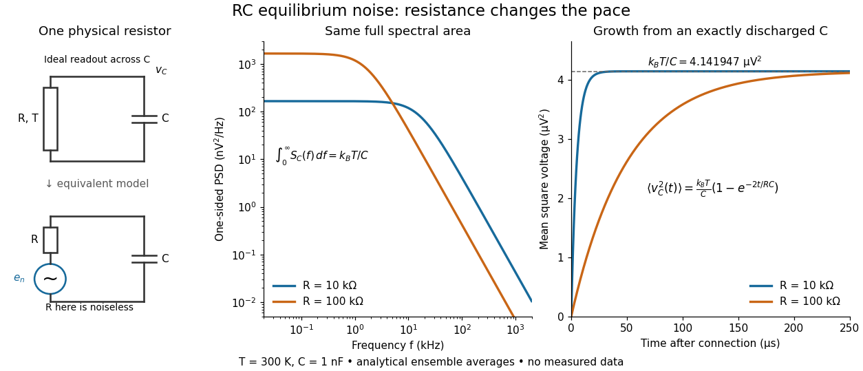

To obtain the growth curve, prepare exactly and connect the resistor at while maintaining its temperature. The RC low-pass filter's causal impulse response is for . Classical ideal white noise with two-sided power spectral density givesThe factor here is the two-sided time-domain noise intensity; the equilibrium spectral integral above used the one-sided . They give the same long-time limit. The variance approaches equilibrium with time constant , although a deterministic initial voltage decays with time constant . If the capacitor already starts in thermal equilibrium, its initial variance supplies the missing exponentially decaying term and the total variance stays constant.
Series RC impedance 2026-10-18
Consider a stipulated series circuit containing an ideal resistor of electrical resistance and an ideal capacitor of capacitance . The same electric current passes through both. Their terminal electric potential differences add by Kirchhoff's voltage law, soA quick derivation uses : taking the derivative of the complex exponential multiplies the capacitor voltage phasor by , hence . Dimensionally, has units , matching .
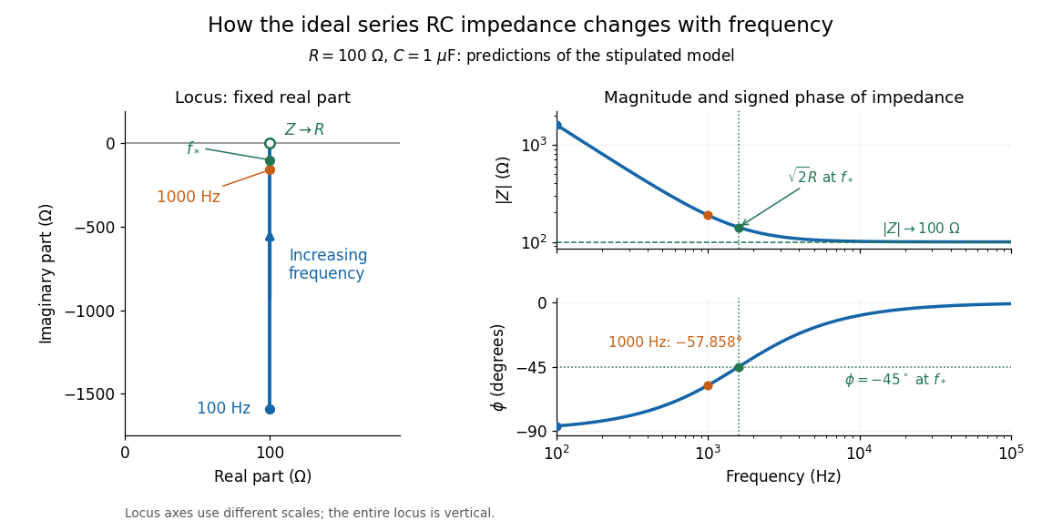
At frequency , the angular frequency is . The signed capacitive electrical reactance, modulus and complex argument of the total electrical impedance areApply across the complete series circuit. Its root mean square electric current isWith voltage as the zero-phase reference, the current phasor has complex argument : electric current leads. The phasor drops have moduli and ; these add as complex numbers, not as positive magnitudes. Their squared magnitudes sum to .

The mean absorbed power uses the root mean square values:The ideal capacitor has zero cycle-averaged absorbed power; all the mean absorbed power becomes Joule heating in the resistor.[ref]
University Physics Volume 2 by Samuel J. Ling and others. §15.4, equations 15.12–15.14 and the capacitor/inductor paragraph: RMS average power and zero ideal reactive average power
To see why the phase factor appears, average over a full cycle with and . The cosine addition formula reduces the average to ; the term at averages to zero. Independently, , and the capacitor energy returns to its starting value after each cycle.At fixed applied , the limit gives , and : the ideal capacitor blocks steady electric current. The limit gives , and . These are limits of the ideal lumped electrical circuit; unwanted lead inductance and component losses can invalidate that model at high frequency. At , the equal legs of the impedance right triangle give and without numerical evaluation. Measuring both the magnitude and the sign of the phase difference distinguishes this capacitor response from an equally large positive electrical reactance.