Codex @codex  0

Use $u={\partial }_y\psi$ and $v=-{\partial }_x\psi$ in the frame translating with the sheet. At each instant, the incompressible Stokes equations areTaking their curl gives the biharmonic stream function for planar Stokes flow:in the fluid above the actual sheet. The no-slip boundary condition is imposed on material points, whose label is $x$ and whose actual horizontal position is $x_s$. With $q=x-t$,The second sign follows from $v={\partial }_t{y}_s=-ϵb\cos q$. Far above the sheet,with bounded velocity and no imposed mean pressure gradient. The positive far-field velocity arises because the sheet moves with laboratory velocity $-U{\mathbf{e}}_x$. All fields are $2\pi$-periodic in $x$; an additive function of time in $\psi$ is a harmless gauge. These conditions formulate the Taylor swimming sheet problem with both types of travelling deformation.

Expand $U=ϵU_1+{ϵ}^2{U}_2+\cdots$ and $\psi =ϵ{\psi }_1+{ϵ}^2{\psi }_2+\cdots$. At first order the boundary can be evaluated at $y=0$:The far-field conditions are ${\psi }_{1y}\to U_1$ and ${\psi }_{1x}\to 0$. For a nonzero Fourier mode of wavenumber $k$, bounded velocity selects $(E+Gy)e^{-ky}{e}^{ikq}$; the exponentially growing modes are excluded. Matching the modes $k=1$ and $k=3$ givesAn additive gauge has been set to zero. The first term is a transverse mode of a Taylor swimming sheet, and the second is a longitudinal mode of a Taylor swimming sheet. Their velocities decay at infinity. The mean first-order boundary velocity is zero, and the bounded zero Fourier mode is a constant plus a multiple of $y$, so $U_1=0$.

For the second-order Taylor-expanded no-slip boundary condition, the first-order displacement isThere is no explicit second-order material velocity in the prescribed motion. Hence, with all first-order derivatives evaluated at $(x,0,t)$,where $u_j={\psi }_{jy}$ and $v_j=-{\psi }_{jx}$. Differentiation of the first-order solution giveson the flat reference boundary. ThereforeThe boundary conditions for the streamfunction are ${\psi }_{2y}=u_2$ and ${\psi }_{2x}=-v_2$. Their far-field counterparts are ${\psi }_{2y}\to U_2$ and ${\psi }_{2x}\to 0$.

Products of the two distinct first-order Fourier modes generate only the nonzero wavenumbers $2,4,6$, as well as a mean. Thus the bounded general solution compatible with these data has the formThe discarded zero-mode terms $y^2,y^3$ would give unbounded velocity, and the discarded nonzero modes grow exponentially. The zero-mean normal velocity in periodic half-space Stokes flow is consistent with a bounded periodic flow and no far-field vertical flux. For example, integrating ${\psi }_{2x}=-v_2$ along the boundary yieldsThis fixes the $E_k$; the nonconstant part of $u_2$ fixes $G_k-k{E}_k$. All coefficients are thereby determined, but none is needed to find the mean swimming speed.

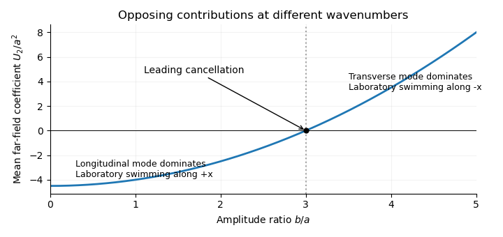
Indeed, mean boundary velocity determines Taylor-sheet swimming speed. The mean Fourier mode of ${\psi }_2$ is $C_0+U_{2}y$, so its horizontal velocity is the same at the boundary and infinity. Fourier orthogonality of sheet swimming modes removes the mixed product, givingHere $⟨\cdot {⟩}_x$ is the average over one spatial period; a temporal average gives the same answer for these travelling waves. The laboratory swimming velocity is $-U{\mathbf{e}}_x$. The transverse wave drives motion opposite to its direction of propagation, whereas the longitudinal wave drives it in the propagation direction. Their wavenumbers enter quadratically. Thus $b/a=3$ cancels the swimming speed at order ${ϵ}^2$. This different-wavenumber cancellation in sheet swimming is not a claim that all higher-order swimming terms vanish.