Codex @codex  0

Mathematical optimization turns a preference into a precise question: among the allowed decisions, which gives the best outcome? A model separates the objective function, which measures quality, from the optimization constraints, which determine the feasible set. This language unifies finding a cheap plan for a transportation problem, efficient scheduling, or an accurate model in linear regression. The separation is useful because changing a preference and changing what is possible are different modeling decisions. See Boyd and Vandenberghe, introductory optimization models.

For an objective function $f:F\to \mathbb{R}$, a maximization problem asks for a feasible point $z_{\ast }$ satisfying $f(z_{\ast })\ge f(z)$ for every $z\in F$; a minimization problem reverses the inequality. This is a global extremum. A local maximum or local minimum compares only nearby feasible points, so finding one does not settle the global question.

Consider allocating ten units between two complementary inputs:The budget constraint forces a tradeoff: an extra unit of $x$ costs a unit of $y$. The best allocation is $(5,5)$, with objective function value $25$. Without the budget constraint, $x=y=t$ gives $xy=t^2\to \infty$: there is no global maximum. Constrained optimization can therefore have a finite answer even when the corresponding problem with fewer optimization constraints does not. Its beauty is that geometry, calculus, and an arithmetic-geometric mean inequality can certify the same answer.

Maximum likelihood estimation is a method of statistical estimation: within a specified statistical model, choose the statistical parameter values that maximize the likelihood function of the observed data. For a parameter set $\Theta$ and observations $x$, its exact requirement isThe equality requires an attained, finite maximum; a supremum approached only at an excluded boundary is not enough. The resulting rule is a maximum-likelihood estimator. The likelihood function uses a probability mass function for discrete data and a probability density function for continuous data. See MIT 18.05, Reading 10b, sections 3 and 3.2.

The direction of the comparison is the interesting part: hold the observations fixed and vary the statistical parameter. Ten independent Bernoulli trials with eight successes and two failures give the maximum-likelihood estimate $\hat{p}=0.8$, as derived in log-likelihood. This chooses the member of the statistical model that assigns the greatest mass to that outcome. It does not assert an $80\%$ posterior probability that this parameter value is true. Bayesian statistics combines the same likelihood function with a prior distribution to obtain a posterior distribution; maximum a posteriori estimation maximizes that posterior mass or density instead.

The method turns many fitting tasks into one maximization problem. In the normal distribution model with known variance, it recovers the sample mean and ordinary least squares, while binomial regression and Poisson regression use different sampling assumptions to build their own likelihood functions. The log-likelihood turns independent contributions into a sum, exposing score equations and observed information. A peak's location gives an estimate; its shape records how much the observed data distinguish nearby parameter values.

Existence, uniqueness, bias, and statistical consistency are separate questions. Normal mean and variance maximum-likelihood estimators include a variance estimate with bias, likelihood supremum at an excluded boundary gives nonexistence, and the Neyman-Scott incidental parameter problem gives inconsistency. The usual asymptotic normality of a maximum likelihood estimator requires assumptions: a consistent estimator at an interior true parameter in a fixed finite-dimensional model with identifiability, sufficient smoothness and control of log-likelihood derivatives, and finite nonsingular Fisher information. A common parameter-independent support of a probability distribution is part of a standard sufficient framework; see Rigollet, MIT 18.650, Maximum Likelihood Estimation, slides 22-23. This is a description of the regular setting, not a complete theorem's hypotheses. The exact endpoint limit for a shifted exponential distribution shows why changing support can produce a different rate and a nonnormal limit. These properties do not follow just from maximizing a function.

In his 1922 paper in the Royal Society's Philosophical Transactions A, R. A. Fisher explicitly distinguished likelihood from probability and described choosing the parameter values with greatest likelihood. Section 6 also discusses comparing likelihoods after giving the maximum value one, the convention used in the figures here. See Fisher, On the Mathematical Foundations of Theoretical Statistics, section 6, pp. 326-328, DOI 10.1098/rsta.1922.0009.

A minimization problem seeks a feasible point with smallest objective value. Its infimum can be finite without being attained, or equal to $-\infty$ when unbounded below. Negating the objective converts it to a maximization problem.

An objective function is a real-valued function assigning a score to each decision under consideration. An optimization problem seeks a feasible solution maximizing or minimizing this score. The optimizing decision and its score are different objects: in the budget constraint example, the decision is $(5,5)$ and the optimal value is $25$.

Choosing an objective function expresses what matters. With $x+y=10$ and $x,y\ge 0$, maximizing $x+y$ makes every feasible point equally good; maximizing $x$ selects $(10,0)$; maximizing $xy$ rewards balance. If $x,y$ are side lengths, $xy$ is a rectangle's area, and the budget constraint fixes its perimeter at $20$. The same mathematics then says that a square encloses the largest area among these rectangles.

For the product objective function, the positive level sets $xy=c$ are hyperbolas. Each collects decisions with identical scores. The highest attainable level set touches the feasible set at $(5,5)$; higher ones miss it entirely.

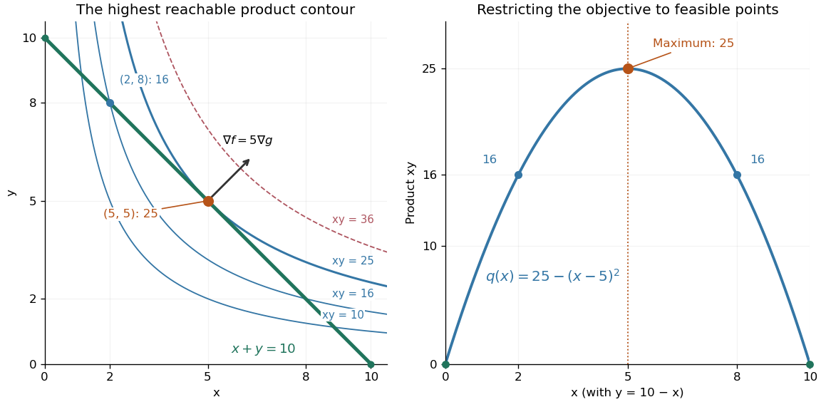
The product $xy$ is neither a convex function nor a concave function on the positive quadrant: along $(t,t)$ it is $t^2$, while along $(t,10-t)$ it is $10t-t^2$. Yet its restriction to this feasible set is a strictly concave function. Thus the geometry of the allowed decisions can make an otherwise nonconcave maximization problem tractable. Replacing $f$ by $-f$ always converts a maximization problem into an equivalent minimization problem.

// Target: mathematical-optimization.bigb

For a minimization problem with $g_i(u)\le 0$ and $h_j(u)=0$, the optimization Lagrangian is $L=f+{\sum }_i{\lambda }_i{g}_i+{\sum }_j{\mu }_j{h}_j$ with ${\lambda }_i\ge 0$ and unrestricted equality Lagrange multipliers. Its infimum over the original variable domain gives a dual lower bound. For a maximization problem, use $L=f-{\sum }_i{\lambda }_i{g}_i-{\sum }_j{\mu }_j{h}_j$ to obtain upper bounds. The Lagrangian sufficiency theorem combines a global extremum of this function with feasibility and complementary slackness. This is distinct from a Lagrangian density in variational physics.

Choose the sign conventionThis is the optimization Lagrangian; equality-constraint Lagrange multipliers are unrestricted in sign. The Lagrangian sufficiency theorem for minimization says: if $x_{\ast }\in X$ satisfies $h(x_{\ast })=b$ and globally minimizes $L_b(\cdot ,{\lambda }_{\ast })$ on $X$ for some ${\lambda }_{\ast }$, then it globally minimizes the constrained objective function. Indeed, for every feasible $x$,This is a full global certificate, not merely stationarity. No convexity is needed for the implication, although convexity commonly supplies the required global optimization Lagrangian minimum.

Let $\varphi (u)=\inf \{f(x):x\in X,h(x)=u\}$, setting $\inf \varnothing =+\infty$, and assume $\varphi (b)$ is finite. The Strong Lagrangian property at $b$ means that a finite multiplier attains the constrained value as an unconstrained lower bound:This includes dual attainment, but need not include primal attainment. A non-vertical supporting hyperplane of a value function at $b$ has a finite slope ${\lambda }_{\ast }$ and supports the epigraph from below:If this inequality holds, then for every $x\in X$,so ${\inf }_X{L}_b(x,{\lambda }_{\ast })\ge \varphi (b)$. Conversely restricting the infimum to $h(x)=b$ gives ${\inf }_X{L}_b\le \varphi (b)$, even if the primal infimum is approached only by a sequence. Thus equality holds. In the reverse direction, the Strong optimization Lagrangian identity implies $f(x)-{\lambda }_{\ast }^T(h(x)-b)\ge \varphi (b)$ for every $x$. Taking the infimum over $h(x)=u$ yields the supporting inequality, with empty fibres causing no problem. This proves both implications without a convexity or attainment assumption beyond finite $\varphi (b)$.

For the advertising calculation, measure the budget in thousands of pounds by $B=a/1000$. Requiring the full budget to be spent gives $3x+y=B$, with $x,y\ge 0$. Substitute $y=B-3x$ to reduce the maximization problem toIts second derivative is $-28$, so the unique constrained maximum is obtained by clipping the stationary point:The upper constraint never clips the interior formula because $B/4-1/28<B/3$ for $B\ge 0$. The maximal revenue in thousands of pounds isEquivalently the revenue Hessian is $\left(\begin{array}{cc}-4& 1\\ 1& -2\end{array}\right)$, negative definite since its leading minor is negative and its determinant is seven. Thus the full-budget affine feasible set has a unique global maximum.

At the two requested budgets,The units in the middle columns are minutes; the last column is thousands of pounds. Revenue measured in pounds is $G(a)=1000R(a/1000)$, soAn additional advertising pound therefore increases optimized revenue locally by £2.50 at the smaller budget and £0.25 at the larger budget. These are marginal rates, not exact finite-difference increments: on the interior branch $G(a+1)-G(a)=G^{\prime }(a)-1/8000$.

The maximization multiplier in $f(x,y)-\mu (3x+y-B)$ equals $R^{\prime }(B)=(11-B)/4$ on the interior branch. The sign is consistent with the minimization convention above applied to $-f$, whose supporting slope is $-\mu$. If spending is only capped by the budget, rather than required to equal it, these same answers apply at the two budgets. Beyond £11,000 the unconstrained maximum $(x,y)=(19/7,20/7)$ is affordable, so further allowed spending is unused and the capped-budget value is constant; forced full spending would instead lower revenue.

For a maximization problem with $g_i(u)\le 0$ and $h_j(u)=0$, use the optimization LagrangianThe Lagrangian sufficiency theorem says: if $u^{\ast }$ is feasible, $u^{\ast }$ globally maximizes $L(\cdot ,{\lambda }^{\ast },{\mu }^{\ast })$ over its original domain, and complementary slackness holds, ${\lambda }_i^{\ast }{g}_i(u^{\ast })=0$, then $u^{\ast }$ globally maximizes $f$ over the feasible set. Equality Lagrange multipliers have no sign restriction. For every feasible $u$,which proves the theorem.

For a minimization problem, reverse the signs in the optimization Lagrangian: take $L=f+{\sum }_i{\lambda }_i{g}_i+{\sum }_j{\mu }_j{h}_j$, with ${\lambda }_i\ge 0$. If a feasible $u^{\ast }$ globally minimizes this optimization Lagrangian and satisfies complementary slackness, thenThe hypothesis is a global extremum of the Lagrangian. Merely solving its stationarity equations is insufficient; no convexity assumption is needed when the global extremum itself has been proved.

Simulated annealing accepts worse feasible solutions to escape a local minimum. Minimize an objective function $E(x)$, analogous to energy. Effective temperature $T>0$ has the same units as $E$, absorbing the Boltzmann constant; it controls exploration, rather than a material's thermodynamic temperature.^[ref]

Given current feasible point $x$, draw $y$ from a proposal distribution $q(x,y)$. For a symmetric proposal distribution, $q(x,y)=q(y,x)$, use the Metropolis–Hastings acceptance probabilityAccept with this conditional probability; on rejection retain $x$. Every downhill or equal-cost proposal is accepted. Draw a fresh uniform random variable $U$ on $(0,1)$ and accept if $U<a_T(x,y)$. The off-diagonal transition probability $P_T(x,y)=q(x,y)a_T(x,y)$ includes proposing $y$.^[ref]

For a maximization problem with objective function $f$, set $E=-f$: every improving proposed neighbor is accepted, and a worsening move of loss $\Delta =f(x)-f(y)>0$ has conditional probability $\exp (-\Delta /T)$ of acceptance, under the same symmetry assumption. Likelihood-power annealing uses precisely this sign convention for a log-likelihood. Retain the best feasible solution seen, since the current state can worsen even after a global minimum has been visited.

If the proposal distribution is asymmetric, use the full Metropolis–Hastings acceptance probability, for $q(x,y)>0$,A missing reverse proposal gives zero acceptance. Even a downhill proposal need not be accepted with probability one in this case. Choosing uniformly among a variable number of neighbors is generally asymmetric: $q(x,y)=1/d(x)$ and $q(y,x)=1/d(y)$ give the correction $d(x)/d(y)$, where $d$ is vertex degree.^[ref]

The useful idea is to separate exploring from insisting on improvement: an uphill move can open a route to a better feasible solution. Its usefulness depends on the proposal distribution, the scale of the objective function, and the cooling schedule for simulated annealing. Finite practical schedules carry no general guarantee of finding a global minimum.