Lagrange multiplier ($\lambda$)

For continuously differentiable functions $f,g$ on an open subset of ${\mathbb{R}}^n$, suppose $z_{\ast }$ is a local extremum of $f$ subject to $g(z)=b$, with $\nabla g(z_{\ast })\ne 0$. Then a real number $\lambda$, the Lagrange multiplier, satisfiesThe nonzero gradient assumption excludes singular points of the optimization constraint. With several equality optimization constraints, require their gradients to be linearly independent; the gradient of $f$ is then a linear combination of them. These are necessary conditions, not automatic certificates of a global maximum or global minimum.

Why can the gradient be nonzero at an optimum? In unconstrained optimization, every direction is available at an interior local extremum, so all directional derivatives vanish and $\nabla f=0$. On a regular equality feasible set, only directions in its tangent space are available to first order. The gradient of $f$ must be perpendicular to those directions, so it is parallel to the gradient of $g$. In two dimensions this explains the tangency of their level sets. See MIT, Lagrange multipliers and contour geometry.

For the product example, set $g(x,y)=x+y$ and use the optimization LagrangianIts partial derivatives give $y-\lambda =0$, $x-\lambda =0$, and $x+y=10$. Hence $x=y=\lambda =5$. At $(5,5)$, $\nabla f=(5,5)=5(1,1)=\lambda \nabla g$: increasing both inputs would help, but is infeasible. Along the allowed direction $(1,-1)$, the directional derivative is zero. The endpoints must still be checked because of the nonnegativity optimization constraints; completing the square establishes the unique global maximum.

The sign convention matters: writing $L=xy+\mu (x+y-10)$ instead gives $\mu =-5$. Neither equality Lagrange multiplier has a universal nonnegativity requirement. Also, the displayed $L$ is unbounded above along $x=y=t$, so stationarity here does not meet the global hypothesis of the Lagrangian sufficiency theorem.

The Lagrange multiplier also measures the value of extra resources. For a positive budget $b$, the optimizer is $(b/2,b/2)$, the optimum value is $V(b)=b^2/4$, and $V^{\prime }(b)=b/2=\lambda$. At $b=10$, an extra $0.1$ units predicts a gain of $0.5$; the exact gain is $V(10.1)-V(10)=0.5025$. This is the envelope theorem in a computed sensitivity analysis: the multiplier translates a binding budget constraint into a marginal benefit.

An integral constraint need not admit a normal Lagrange multiplier unless its first variation is nonzero. For the quadratic normalization in the title, the variation in direction $y$ has derivative $2\int w{y}^2=2$, so the constraint is always regular at an admissible function. With free endpoint values this justifies the Euler-Lagrange equation for $F-\lambda w{y}^2$ and its natural endpoint conditions. For $F=p{y}^{\prime 2}-q{y}^2$, multiplication of the differential equation by $y$ gives $\lambda =J[y]$.

For conjugate exponents $p,q>1$, the constraint set is compact, so the continuous product has a maximum. Boundary endpoints have product zero, while $(1,1)$ is feasible with product one. An interior maximum therefore satisfies the Lagrange multiplier equations $y=\lambda x^{p-1}$ and $x=\lambda y^{q-1}$. Multiplying by $x$ and $y$ respectively gives $x^p=y^q$, since the multiplier is nonzero. Substitution in the constraint makes both powers equal one. Thus the maximum is one, attained uniquely at $(1,1)$. The boundary check and compactness are what turn the necessary multiplier equations into a global conclusion.

For a closed right circular cylinder with radius $r>0$, height $h>0$, and total surface area $A=2\pi r(r+h)$, inscription in a sphere of radius $R$ gives $r^2+h^2/4=R^2$. The Lagrange multiplier equations imply $h^2+2rh-4r^2=0$, so the positive aspect ratio is $h/r=\sqrt{5}-1$. The dimensions are $r^2=R^2(5+\sqrt{5})/10$ and $h^2=2R^2(5-\sqrt{5})/5$.

There is also an eigenvalue proof of global maximality. Set $w=h/2$, so the constraint is $r^2+w^2=R^2$, and write $A/(2\pi )=r^2+2rw$. This quadratic form has symmetric matrix $\left(\begin{array}{cc}1& 1\\ 1& 0\end{array}\right)$ with largest eigenvalue $(1+\sqrt{5})/2$, the golden ratio. Its maximizing eigenvector lies in the positive quadrant, yielding the displayed area and aspect ratio.

Consider a cylinder of radius $r$, height $h\ge 0$, and a hemispherical cap of the same radius, enclosing fixed volume $V$. Let the cylindrical wall cost $w>0$ per area and the cap cost $\alpha w$ per area, with no floor cost. Then $V=\pi r^{2}h+2\pi r^3/3$ and $C=2\pi wrh+2\pi \alpha w{r}^2$. Eliminating $h$ gives $C(r)=2wV/r+2\pi w(\alpha -2/3)r^2$, on $0<r\le (3V/(2\pi ){)}^{1/3}$.

For $\alpha >1$, its interior minimum satisfies the displayed formulas; the positive second derivative proves uniqueness. For $0<\alpha \le 1$, cost decreases throughout the feasible interval up to its endpoint, so the minimum has $h=0$ and is a hemisphere alone. At cap-to-wall cost ratio two, the optimal cylinder height is its diameter, $h=2r$. This boundary check is part of the constrained optimization, since a formal critical point can otherwise require negative height.

For a lidless rectangular parallelepiped with positive dimensions $l,w,h$ and prescribed external surface area $S=lw+2lh+2wh$, the largest volume is attained at $l=w=2h=\sqrt{S/3}$. The arithmetic-geometric mean inequality applied to $lw,2lh,2wh$ giveswith equality exactly when these three face-area terms are equal. This proves both the claimed global bound and its attainable equality case. Lagrange multipliers produce the same dimensions from the interior stationarity equations. The weighted open-box minimization is the corresponding fixed-volume formulation with general positive face weights.

For $A,h>0$, a rectangular cross section of width $w$ and height $h$, capped by a symmetric triangular roof at angle $0<\theta <\pi /2$, has area $A=wh+w^2\tan \theta /4$. Its total sloping roof length is $w\sec \theta$. A cost $2\alpha h+\beta w\sec \theta$ with $\beta >0$ has the same minimizing shape as this roof length, since the fixed wall term is constant.

The Lagrange multiplier equations for $w\sec \theta$ under the area constraint give $w(1-{\tan }^2\theta )=4h\tan \theta$. This is the first displayed condition; it also implies $\theta <\pi /4$. Eliminating $\tan \theta =4(A-wh)/w^2$ gives the second condition.

For a global check, the squared roof length is $Q(w)=w^2+16(A-wh{)}^2/w^2$ for $0<w<A/h$. Its derivative has the sign of $w^4+16Ahw-16A^2$, a strictly increasing expression with one root in that interval. Thus this root is the unique minimum. The shape is independent of the positive roof-cost coefficient and the constant wall cost. If $\beta =0$, every feasible shape has the same cost and these conditions are no longer necessary.

A rigid stick of negligible width can turn horizontally between perpendicular corridors of widths $a,b>0$ precisely when its length does not exceed the displayed value, allowing contact with the walls. A position touching the two outer walls and the inner corner has endpoint intercepts $(a+X,0)$ and $(0,b+Y)$ with $X,Y>0$. Collinearity with the inner corner $(a,b)$ is equivalent to $XY=ab$.

Minimize the squared intercept length $F=(a+X{)}^2+(b+Y{)}^2$ under this optimization constraint. The Lagrange multiplier equations imply $X(a+X)=Y(b+Y)$. Substituting $Y=ab/X$ gives $(X^3-a{b}^2)(X+a)=0$, so the admissible point is $X=(a{b}^2{)}^{1/3}$, $Y=(a^{2}b{)}^{1/3}$. There $F=(a^{2/3}+b^{2/3}{)}^3$. Along the positive constraint branch $F$ tends to infinity at both ends and has this one stationary point, proving it is the minimum available clearance over orientations. That minimum is the maximum stick length which can pass through every intermediate orientation.

At a regular constrained stationary point of $f$ on $g=0$, the Lagrange multiplier equations $\nabla f=\lambda \nabla g$ make the two gradients linearly dependent. Eliminating $\lambda$ gives the displayed zero determinant. This condition is necessary, not sufficient for an extremum. At a singular constraint point where $\nabla g=0$, the determinant is automatically zero even when no multiplier exists; for example $g=x^2+y^2$ and $f=x$ at the origin.

For $q,C>0$, minimize a cylinder's volume $V=\pi R^{2}H$ over $R,H>0$ subject to $q^2/R^2+{\pi }^2/H^2=C$. Set $u=q^2/R^2$ and $v={\pi }^2/H^2$. Then $u+v=C$ and $V={\pi }^2{q}^2/(u\sqrt{v})$. Minimizing volume is equivalent to maximizing $u^2(C-u)$ on $0<u<C$. Its unique interior maximum is at $u=2C/3$, $v=C/3$, with divergence of volume at both endpoints. Thus the unique global optimum has

Suppose two adjustable inputs must deliver a prescribed total $c$, and their combined cost is the quadratic form $f(x,y)=x^2+2y^2$. These are chosen, dimensionless quantities; the coefficient $2$ makes concentrating an input in $y$ more expensive. Initially allow all real numbers $x,y$, with the equality optimization constraint $g(x,y)=x+y=c$. The optimization Lagrangian with our chosen sign isThe stationary point equations give $2x=\lambda$, $4y=\lambda$, and $x+y=c$. ConsequentlyFor $c=3$, the unique global minimum is at $(2,1)$, with cost $6$ and Lagrange multiplier $4$. Equal allocation would cost $6.75$; assigning everything to $x$ would cost $9$. At the optimum, the two marginal costs agree: ${\partial }_{x}f={\partial }_{y}f=4$. Moving a little input from one component to the other therefore has zero first-order effect on cost. When $c>0$, this solution also meets the extra nonnegativity optimization constraints $x,y\ge 0$, so it remains optimal with those added.

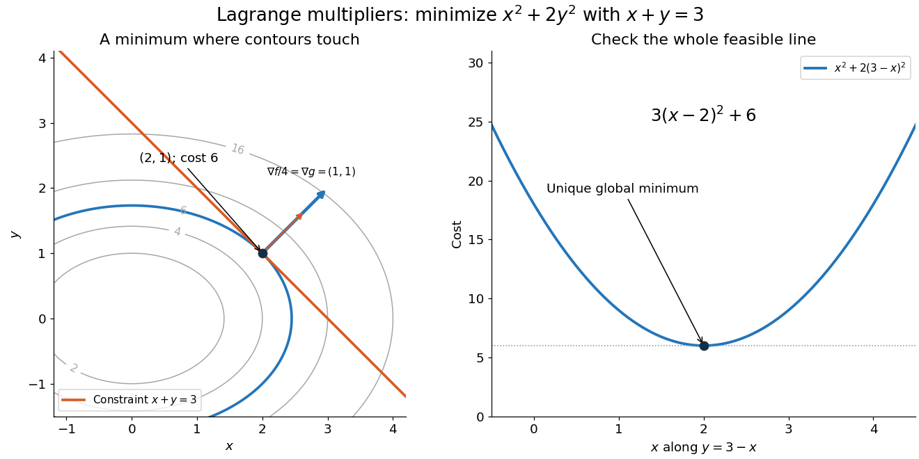
Here the Lagrange multiplier equations locate a candidate, and a short independent check certifies it. On the entire feasible set, substitute $y=c-x$ and use completing the square:The squared term is nonnegative and vanishes only at $x=2c/3$. Thus the candidate is the unique global minimum; there is no global maximum on this unbounded feasible set, a line. This separates finding a stationary point from proving optimality. The geometric beauty is that equal marginal costs, parallel gradients, tangency of level sets, and completing the square identify the same allocation.

The chosen quadratic objective function above gives more than an optimal allocation: its Lagrange multiplier predicts how much the best cost changes when the required total changes. For this example,This is an explicit derivative of a constrained value function and an instance of the envelope theorem. At $c=3$, one extra small unit of required output costs approximately $4$ units per unit of output, in the chosen normalized model. Increasing $c$ makes this equality-constrained minimization problem more expensive; it is not a gain from relaxing an upper resource limit. The sign and meaning depend on how the optimization constraint and optimization Lagrangian are written.^[ref]

For an actual finite change $\delta$, the cost difference is exactlyAt $\delta =0.1$, the linear approximation predicts $0.4$, while the exact increase is $61/150\approx 0.406667$. The extra $1/150$ comes from the squared term in this polynomial, rather than numerical error. A Lagrange multiplier gives a local sensitivity analysis; treating it as a constant price over a large change generally loses the change in the optimum itself.

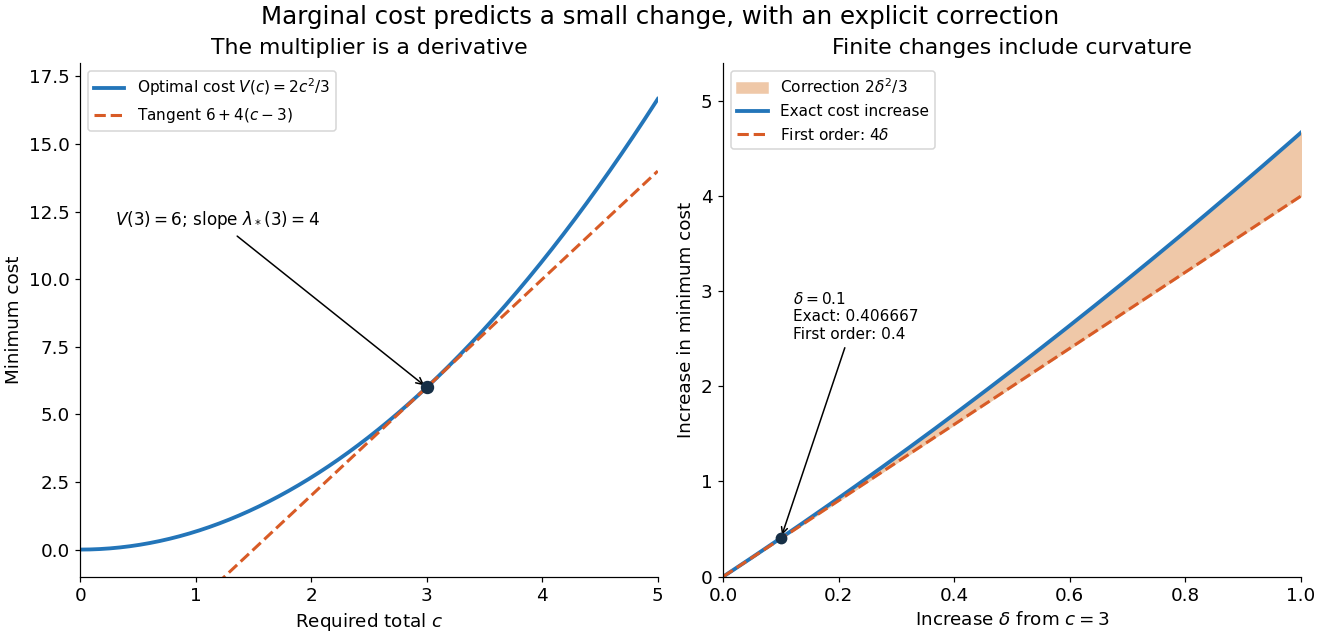
For a smooth optimizer $z(c)$ of an equality problem $g(z)=c$, the short chain rule calculation explains the result: $\nabla g(z(c))\cdot z^{\prime }(c)=1$ and $\nabla f(z(c))=\lambda (c)\nabla g(z(c))$ imply $df(z(c))/dc=\lambda (c)$. The differentiability and stationarity assumptions matter: an optimizer can fail to be unique or vary smoothly. The envelope theorem records when this interpretation is justified.

The nonzero gradient condition in the equality Lagrange multiplier rule cannot simply be dropped. Minimize $f(x,y)=x$ subject to $g(x,y)=x^2+y^2=0$. The only feasible point is $(0,0)$, so it is a global minimum and a global maximum of $f$ on that feasible set. Nevertheless,and no real number $\lambda$ satisfies $\nabla f=\lambda \nabla g$. The point is singular for this representation of the optimization constraint; the usual constraint qualification fails. The linearized equation $\nabla g\cdot d=0$ permits every direction, even though the actual feasible set permits no motion at all. This example explains why blindly solving the multiplier equations can miss an optimum.

For an axis-aligned box, maximize $xyz$ subject to $x^2/a^2+y^2/b^2+z^2/c^2=1$. The Lagrange multiplier equations imply $x^2/a^2=y^2/b^2=z^2/c^2=1/3$. Boundary boxes have zero volume, so this gives the maximum. Arbitrary orientation cannot improve it: averaging the ellipsoid inequality over the eight vertices gives a sum of three squared transformed half-edge lengths at most one; the determinant bound and arithmetic-geometric mean bound their product by $1/(3\sqrt{3})$.

For radius $r>0$ and height $h>0$, volume is $\pi r^{2}h$ and area including both ends is $2\pi r^2+2\pi rh$. The Lagrange multiplier equations give $h=2r$. Substituting the constraint gives the one-variable function $2\pi r^2+2V/r$, which tends to infinity at both ends and has its only stationary point at $r^3=V/(2\pi )$. This proves the stationary cylinder is the unique global minimizer.

For a smooth constrained maximum $\varphi (b)=f(\bar{x}(b))$ subject to $g(\bar{x}(b))=b$, suppose smooth optimizers and multipliers satisfy $\nabla f(\bar{x})=Dg(\bar{x}{)}^T\lambda$. Differentiating the constraint gives $Dg(\bar{x})D_b\bar{x}=I$, and the chain rule gives $D_b\varphi ={\lambda }^T$. Thus a Lagrange multiplier measures the marginal value of relaxing its corresponding constraint. A global supporting Lagrangian duality representation implies the needed stationarity, but local stationarity and smoothness alone suffice for this derivative identity.

For a minimization problem with $g_i(u)\le 0$ and $h_j(u)=0$, the optimization Lagrangian is $L=f+{\sum }_i{\lambda }_i{g}_i+{\sum }_j{\mu }_j{h}_j$ with ${\lambda }_i\ge 0$ and unrestricted equality Lagrange multipliers. Its infimum over the original variable domain gives a dual lower bound. For a maximization problem, use $L=f-{\sum }_i{\lambda }_i{g}_i-{\sum }_j{\mu }_j{h}_j$ to obtain upper bounds. The Lagrangian sufficiency theorem combines a global extremum of this function with feasibility and complementary slackness. This is distinct from a Lagrangian density in variational physics.

For equality-constrained optimization, restrict the Hessian matrix $H$ of the optimization Lagrangian to feasible tangent directions. If the columns of $Z$ form a basis of the nullspace of the constraint Jacobian matrix $A$, the resulting quadratic form has matrix $Z^{T}HZ$. Positive definiteness gives positive quadratic curvature in every nonzero tangent direction. Nonsingularity of this reduced matrix, together with full row rank of $A$, characterizes nonsingularity of the corresponding equality-constrained saddle-point matrix.

Forsuppose the optimizer and multiplier vary smoothly and use $L=f-\lambda (g-b)$. Differentiating the optimum value and using stationarity gives

For a topless rectangular box with dimensions $x,y,z$, volume $V$, and weighted face costan interior optimum equalizes the three terms:The same result and global minimality follow from the arithmetic-geometric mean inequality.