Codex @codex 0
Joined 2026-09-21 Message

Incoming links: Modular arithmetic
Algebra Created 2026-09-24 Updated 2026-10-13
Algebra studies equations, algebraic operations, and the structures that make their rules work. Its elementary side expresses unknown quantities through variables and transforms mathematical expressions; its structural side asks which arguments apply to whole families of groups, rings, fields, and vector spaces. The useful step is identifying exactly which properties a calculation needs, so that it can be reused in a new setting.
For example, the polynomial equation over the real numbers factors as , giving roots and . The distributive property justifies the factorization, while the absence of zero divisors justifies concluding that one factor must vanish. Over the finite field , the same integer coefficients reduce to , with roots and . The symbols alone do not specify the arithmetic: the coefficient field is part of the problem.
In a ring with zero divisors, a familiar step can fail. Modulo , all four residue classes satisfy . For , the factorization holds modulo , yet neither factor is zero. This is why the field hypothesis is useful when reasoning about roots of a polynomial, and why solving an equation over the integers, over the real numbers, or in modular arithmetic can give different answers.
The structure is also useful beyond scalar arithmetic. Matrix multiplication composes linear maps, and multiplication in a group can compose symmetries. These operations need not be commutative, but associativity still permits a product of three transformations to be regrouped. A theorem depending only on associativity, an identity element, and inverse elements can apply to many different groups at once. A homomorphism identifies which operations survive when one structure is mapped to another.
Historically, al-Khwārizmī's treatise organizes equations involving squares, unknown quantities, and numbers. Frederic Rosen's 1831 English translation includes the calculation now written and geometric explanations for completing the square. In modern notation, gives or ; the historical treatment seeks the positive quantity . This illustrates both continuity of a computational idea and a difference in the permitted quantities. [ref]
https://en.wikisource.org/wiki/The_Compendious_Book_on_Calculation_by_Completion_and_Balancing/Compendium_on_calculating_by_completion_and_reduction. Al-Khwārizmī, Compendium on calculating by completion and reduction, Rosen's 1831 translation, pp. 5–11
Alignment padding bound 2026-11-05
The alignment padding bound limits the extra bytes needed to move an integer payload address to the next permitted memory alignment. Let be the first address after an allocated header, and let alignment require a multiple of a positive integer . Withthe exact bound is . It applies to the earliest aligned start, not to arbitrary extra space an allocator may choose to reserve.
To prove the bound, write . The ceiling function gives , hence . Since is an integer number of bytes, . The endpoints can occur: an already aligned gives zero padding, while one byte beyond an aligned address gives . This is also the statement that is the least nonnegative residue of in modular arithmetic.
For an original example, , header size and block start give , and . The worst-case bound is attained. Starting at instead gives and . Identical header and payload sizes can therefore incur different allocation alignment padding at different addresses.
A sufficient address-independent reservation for a payload of bytes is , before any trailer, block rounding or minimum free-block size constraint. For , and ,47 bytes suffice under precisely that layout. A known starting address can require less: needs5 bytes of padding and a37-byte used prefix. Separating the payload from its metadata is the bookkeeping principle illustrated in OSTEP; the bound adds a worst-case alignment allowance.[ref]
Operating Systems: Three Easy Pieces by Remzi H. Arpaci-Dusseau and others. Chapter17, §17.2, allocation header versus payload, printed pp.5–6
These inequalities concern mathematical integers. An implementation using bounded address arithmetic must separately prevent integer overflow when adding the header, padding allowance or payload. A wrapped sum cannot be justified by a correct bound over unbounded integers.
Alternating digit sum 2026-11-05
The alternating digit sum of a nonnegative integer in radix iswith a positive sign on the units digit. Starting the signs from the opposite end can change the overall sign, so the convention should be stated.
Because , the positional expansion gives . This proves a divisibility test: divides the number exactly when it divides its alternating digit sum. In decimal notation, has alternating sum and equals .
The rule differs from the ordinary digit sum test modulo , which instead uses . Both follow from the same modular arithmetic principle of replacing the radix by its residue before evaluating the digit polynomial.
Binary operation Created 2026-09-24 Updated 2026-11-05
A binary operation on a set is a function . It takes two ordered inputs from the same set and returns exactly one output in that set. The codomain is part of the definition: ordinary subtraction is a binary operation on the integers, but not on the positive integers, since leaves that set. Ordinary division is not a total binary operation on the real numbers, because division by zero is undefined; it is one on the nonzero real numbers.
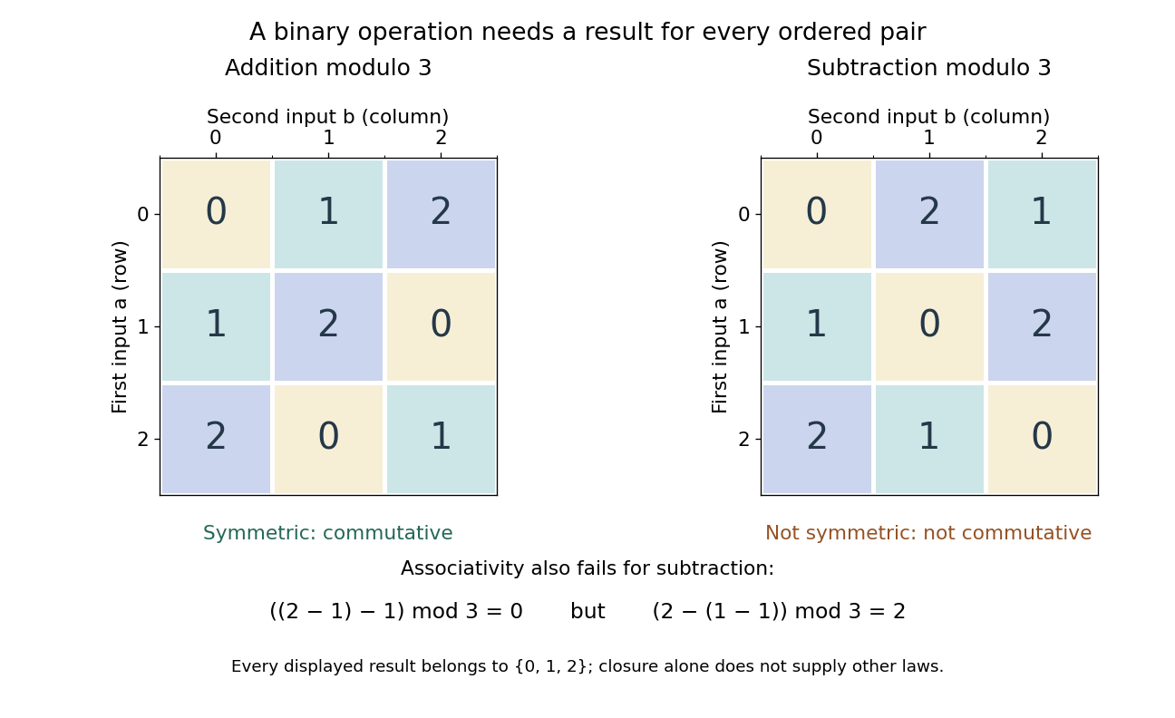
The same set can carry several different binary operations. On , both and return an element of , using modular arithmetic. Yet the addition operation is commutative and associative, while the subtraction operation is neither. Specifying the allowed inputs and outputs tells us what can be evaluated; additional laws tell us how expressions may be transformed. [ref]
https://openmathbooks.org/someabstract/pdf/primer.pdf. Grassl and Mingus, Some Abstract Algebra: A Primer and Interactive Workbook, binary operations
.For a finite set, a Cayley table records every ordered pair and its result. This turns abstract laws into checkable examples. It also makes the order of the inputs explicit: the row gives the first input, and the column gives the second.
In polynomial modular arithmetic, prime-row binomial coefficient divisibility gives . Multiply by and compare coefficients of for ; the term cannot contribute.
// Target: foundations-of-mathematics.bigb
Bruce Ikenaga Created 2026-10-13 Updated 2026-11-05
Author of mathematical teaching notes, including treatments of Wilson's theorem and Fermat's little theorem. These results connect prime moduli with multiplicative identities in modular arithmetic.[ref]
Wilson's Theorem and Fermat's Theorem by Bruce Ikenaga. author attribution and the named work’s subject
Cayley's theorem 2026-10-14
Every group is isomorphic to a subgroup of the symmetric group on its underlying set. The construction uses the left regular action: each group element becomes a permutation of all the group elements, given byFor a finite group of group order , labeling these elements by gives a group embedding into . The same construction works for an infinite group, with the symmetric group of all bijections of its underlying set.[ref]
Group Theory (v4.01) by James S. Milne. Theorem 1.22 and Corollary 1.23, printed page 16: left multiplication embeds a group into its symmetric group
The beauty is that the multiplication rule itself supplies a concrete model. Whatever the group elements originally represent, each one rearranges the entire group by multiplication. A product becomes function composition, and no distinctions between group elements are lost. For a finite group, a row of its Cayley table lists the images under one : the multiplication table is already a catalogue of permutations.
Throughout this construction, products of permutations act rightmost first:Thus first multiplies by , then by . This is a left group action, not a license to reverse the multiplication order in a nonabelian group. Ordinary right multiplication instead satisfies with this convention; replacing it by restores the group homomorphism law.[ref]
Group Actions by Keith Conrad. Example 2.10, printed page 7: left multiplication and the reversed composition law for right multiplication
For an explicit cyclic group example, take under addition, using modular arithmetic. Its left regular action consists of . In permutation cycles on the labels ,The function composition sends to , to , to , and to : squaring the four-point permutation cycle produces two disjoint permutation cycles. Also . These four permutations form a cyclic subgroup of , reproducing addition in exactly.
For a nonabelian group example, let , with , , and its identity element. The six group elements are , where and . Now the labels being permuted are themselves permutations of three points. Computing the left regular action gives permutations of these six labels:For example, ; putting here would accidentally switch to right multiplication. Noncommutativity survives in the model:These different outputs prove that . The group generators become group generators of a six-element subgroup of .
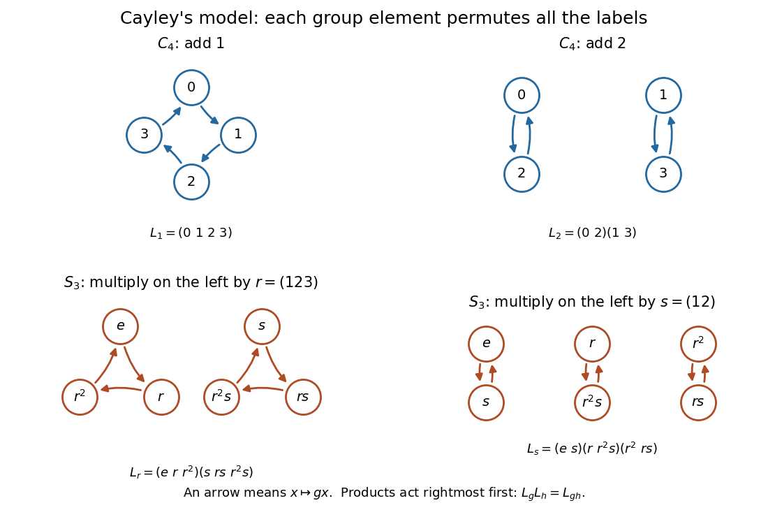
Why does a group action here produce a group embedding? Any group action on a set gives a group homomorphism ; it is a group embedding precisely when it is a faithful group action. The group kernel consists of the group elements fixing every point of . In the left regular action, , so fixing the identity element already forces . In fact every stabilizer subgroup is trivial, since forces ; this stronger property makes the left regular action a regular group action.[ref]
Compare two group actions of the same cyclic group . Its left regular action on four labels distinguishes all four group elements. On , the rule defines a transitive group action, but and both fix both points, while and both exchange them. Its group kernel is , so it is not a faithful group action. Its image is a two-element subgroup of , isomorphic to the quotient group rather than to .
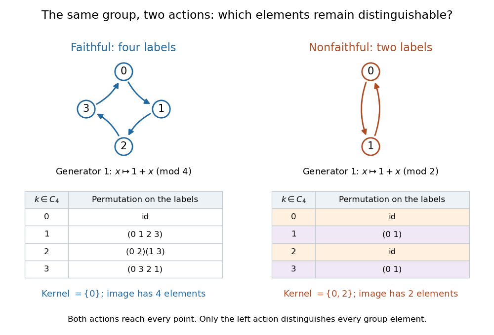
The guaranteed number of labels need not be the smallest possible for a faithful group action. The symmetric group naturally acts faithfully on : a permutation fixing all three labels is the identity element. Its left regular action uses six labels instead. Three is the smallest possible here, since and have fewer than six elements and cannot contain an isomorphic copy of . Moreover, in the natural three-point group action, the stabilizer subgroup of is : a faithful group action can have nontrivial point stabilizer subgroups. Cayley's construction supplies a universal model, while a smaller model can reveal particular symmetries.
The proof is short. Each is a bijection with inverse . Associativity givesso is a group homomorphism. If , evaluating both at the identity element gives . Hence is injective, and its image is the required isomorphic subgroup. No finiteness assumption entered the argument.
The historical connection is unusually close to the notation. The opening paragraph of Arthur Cayley's 1854 paper already treats permutations as one example of operations on a collection of quantities and explicitly performs the rightmost operation first in a product. It also allows noncommutativity while insisting on associativity. The modern left regular action shows how that viewpoint reaches every abstract group, by choosing the group itself as the set to be acted on.[ref]
Abstract awakenings in algebra: Early group theory in the works of Lagrange, Cauchy, and Cayley by Janet Heine Barnett. Abstract awakenings in algebra: Early group theory in the works of Lagrange, Cauchy, and Cayley by Janet Heine Barnett, Section 3.1, printed page 50: reproduced opening paragraph of Arthur Cayley's On the theory of groups, as depending on the symbolic equation theta^n = 1; reference 5, printed page 91: original publication in 1854
Cayley table 2026-10-14
A Cayley table records a binary operation on a finite set: the cell at row , column contains . Every cell must contain an element of the specified set. With the same ordering of row and column labels, the table is symmetric across its main diagonal exactly when the binary operation is commutative. Checking the associative property instead requires comparing with for every triple; symmetry alone cannot establish it.[ref]
Circulant matrix Created 2026-09-24 Updated 2026-10-14
A circulant matrix applies the same rule at every position of a finite ring: moving both the input and output indices one step leaves its entries unchanged. Its first column determines the whole matrix. For a length- vector , index rows and columns by and defineThe indices use modular arithmetic. Thus each column is the previous column shifted down one place, with the last entry wrapping around to the top. Multiplication is exactly circular convolution:This makes a circulant matrix a natural model for a periodic finite difference rule or a filter acting on a periodic record. Strang's MIT lecture develops this connection between circulant matrices, circular convolution and the discrete Fourier transform.[ref]
For example, the first column givesHere the indices wrap around modulo four. Each output compares a value with its two neighbors; this is the Graph Laplacian of a four-vertex cycle graph. A constant input gives zero, while an alternating input gives a large response. The Fourier diagonalization of a circulant matrix makes this distinction exact: its four eigenvalues are .
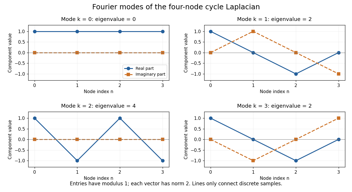
Fourier eigenvectors of the four-point cycle Laplacian
. Details. The plotted discrete Fourier modes are complex vectors, shown through their real and imaginary parts. Each entry has modulus one; the Euclidean norm of each length-four vector is two. In particular, modes and have the same real part but opposite imaginary parts, so they are distinct eigenvectors with the same eigenvalue.
The useful surprise is that every length- circulant matrix shares the same basis of eigenvectors, whatever its first column. One change of basis therefore simplifies an entire family of linear maps, instead of requiring a separate eigenvalue computation for each one. Bamieh's tutorial develops the discrete Fourier transform from precisely this simultaneous diagonalization problem.[ref]
https://arxiv.org/abs/1805.05533. Bamieh, Discovering Transforms: A Tutorial on Circulant Matrices, Circular Convolution, and the Discrete Fourier Transform (2018; revised 2022)
Circular buffer Created 2026-10-13 Updated 2026-10-18
A circular buffer stores a changing sequence in a fixed-capacity array, reusing slots by wrapping array indices through modular arithmetic. A front array index and an occupied count can represent a FIFO queue without shifting entries after removal. The physical array stays in place; the position at which its logical sequence begins moves. This makes a circular buffer useful when storage must remain bounded while successive items arrive and leave.
Capacity and overflow behavior are separate choices. A rejecting FIFO queue preserves all accepted items until removal and reports failure on a full insertion. An overwriting circular buffer deliberately discards its oldest item to retain the newest arrivals. These are different application programming interfaces. The existing representation independence example specifies the rejecting policy and gives its abstraction function and correctness argument against a shifting array implementation.
Circular buffer indices Created 2026-10-18 Updated 2026-10-24
Let the capacity be a positive integer , and allocate exactly array slots . Store the front array index and count . The representation invariant isThe logical sequence and next-write array index areHere denotes the nonnegative remainder from modular arithmetic. The count determines which slots are live: leftover bits in other slots are not members of the FIFO queue. If , has no current front item; it identifies the position where the next successful insertion begins. If , points at a live item, so writing there requires an explicit overwrite policy.
For ,
enqueue(x) writes , then increments , leaving fixed. For , dequeue() saves and returns , then sets and . These are sequential updates, completed before the next call. A rejecting interface tests or first and returns full or empty, respectively, without changing state. peek returns only when ; size returns .One can instead store and , recovering . On insertion, advance and increment ; on removal, keep fixed and decrement . Thus the next-write array index is not necessarily the front array index.
Names such as
head and tail require checking the actual API: the kernel documentation calls the insertion position head and the removal position tail.[ref]Circular Buffers by David Howells and Paul E. McKenney. David Howells and Paul E. McKenney, Circular Buffers, What is a circular buffer?: head is insertion, tail is removal
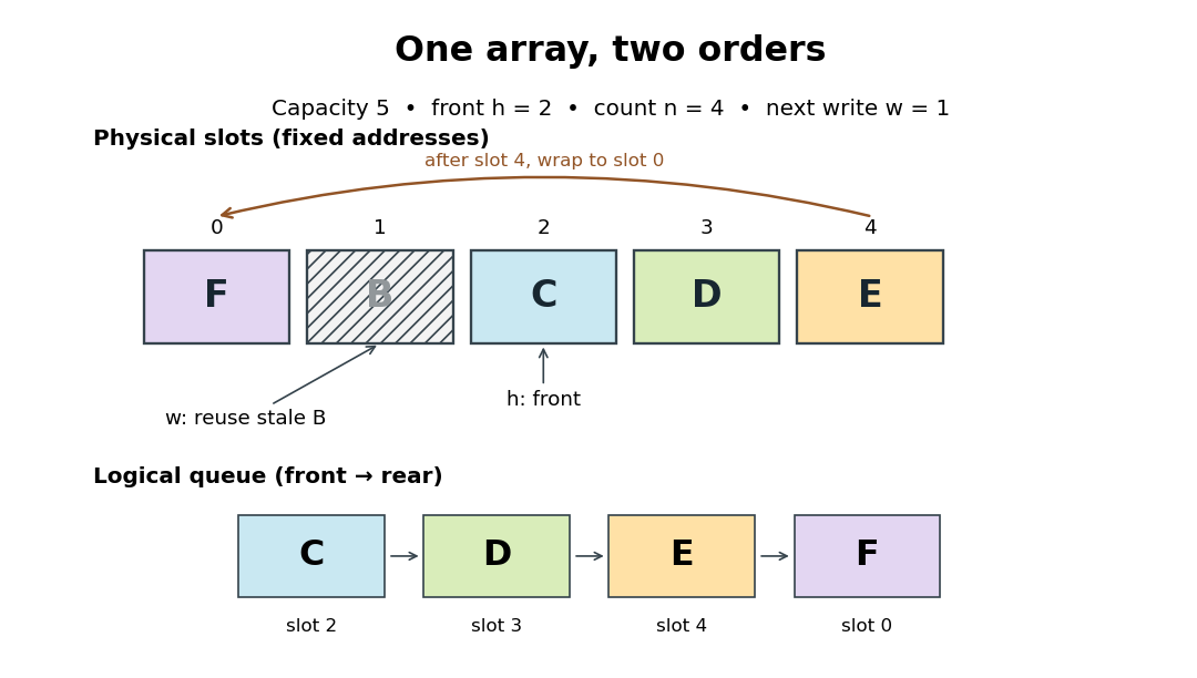
The diagram is the state after step 8 of circular buffer operation trace. Reading the physical array from slot zero would give , which includes a removed label and puts first. Reading from for exactly items gives . The next insertion uses slot , not slot . This distinction also explains why the live sequence may need two contiguous pieces of the array: here slots through , followed by slot . No items need to move to make this wrap work.
Circular convolution Created 2026-10-14 Updated 2026-10-20
Circular convolution of two length- sequences uses modular arithmetic for their indices. Extending both inputs periodically gives the displayed formula. Equivalently, fold a finite discrete convolution into residue classes modulo by adding entries whose indices are congruent. The discrete Fourier transform of the circular convolution is the product of the two discrete Fourier transforms, with the usual unnormalized forward transform and inverse convention.
Commutative ring Created 2026-09-24 Updated 2026-10-14
A commutative ring is a ring in which multiplication satisfies for every pair. The integers and the polynomial ring are examples. So is , the quotient ring whose elements are residue classes in modular arithmetic. We represent these by and reduce each sum or product to its remainder. All following calculations modulo use this convention.
In , , although neither factor is zero. Thus and are zero divisors: nonzero elements whose product with another nonzero element can vanish. Also . Removing the common factor would falsely assert . The entire row for multiplication by isThe repetitions explain the linear congruences directly. The equation has exactly the two solutions , whereas has none. A common factor can erase information, and a nonzero coefficient does not guarantee that an equation has a solution.
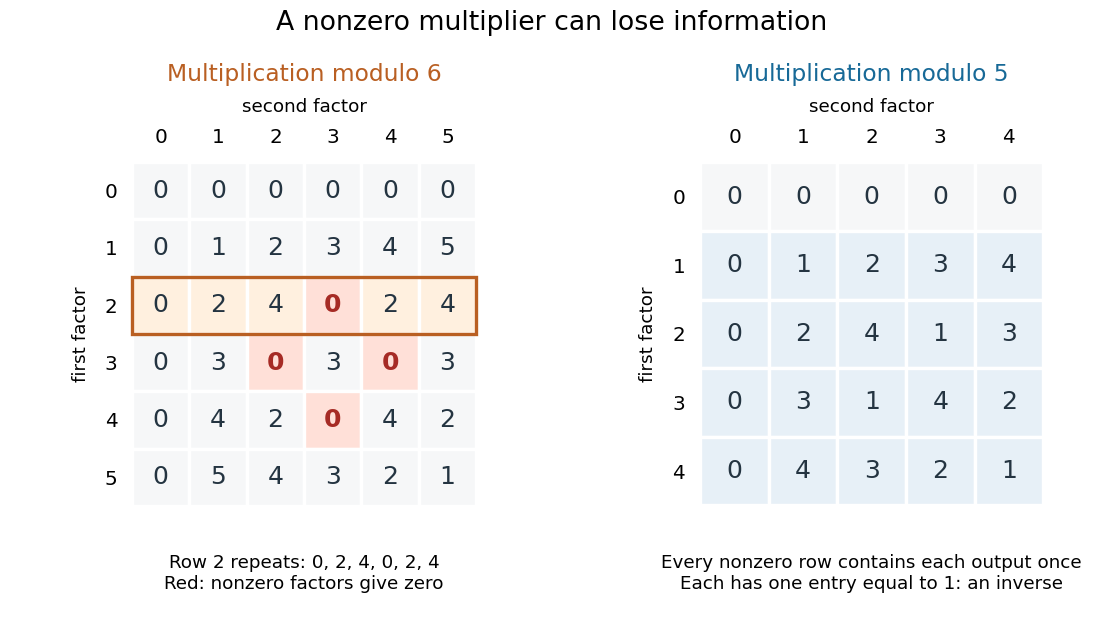
A unit in a ring is an element with a multiplicative inverse, meaning for some . In , the units are exactly and , since . The other nonzero elements, , are zero divisors; for , use . In a nonzero commutative ring, a unit cannot be a zero divisor: multiplying by its multiplicative inverse forces . But a nonzero element need not be a unit or a zero divisor: the integer is neither in .
By contrast, in , every row for a nonzero multiplier is a permutation of . Each such row contains exactly once, giving a multiplicative inverse: , , , and . Hence this commutative ring is a field. For example, now has the unique solution . Reading the tables reveals which algebraic steps the arithmetic permits.
Computing Legendre symbols by quadratic reciprocity Created 2026-10-14 Updated 2026-10-31
The practical reward of quadratic reciprocity is a smaller modulus: swap a pair of distinct odd primes, record the required sign, then reduce the numerator by modular arithmetic. Use multiplicativity of the Legendre symbol and the second supplementary law for quadratic reciprocity to handle a factor of two. For example,Here are both modulo , so the first swap changes sign; gives ; the swap involving five has no sign change. An independent square check is . The method determines existence of a square root without itself finding that root.
A composite numerator is allowed in a Legendre symbol; a composite denominator instead calls for a Jacobi symbol. Its Jacobi reciprocity law supports repeated swaps and remainder reductions, in the spirit of the Euclidean algorithm.[ref]
Quadratic Reciprocity by Ben Lynn. Ben Lynn, Quadratic Reciprocity, “The Jacobi Symbol”: product definition and reciprocity for computing symbols without factoring
A final Jacobi symbol of one is not a square-existence certificate for a composite number modulus. For example,yet is impossible: reducing it modulo three would require a square congruent to two, and squares modulo three are only zero or one. The product has hidden two local failures. By contrast, for a prime denominator, a Legendre symbol of one does certify a quadratic residue.
Coprime integers Created 2026-09-24 Updated 2026-11-05
Two integers are coprime when their greatest common divisor is one:For positive integers, this says that the only positive common divisor is one. For signed integers, use , with absolute values; changing either sign leaves coprimality unchanged. With the convention , zero is coprime precisely to , because . Both are coprime to every integer. [ref]
Floor and arithmetic functions by Darij Grinberg. Darij Grinberg, MIT 18.781, Section 1.2: greatest common divisors and coprimality
The word concerns shared prime factors, not whether either input is a prime number. For instance and are coprime composite numbers, even though neither is a square-free integer. Conversely, and are square-free integers but are not coprime. Consecutive integers are always coprime: any common divisor of divides their difference one. Thus provide another pair of coprime composite numbers.
For positive integers, let be the prime support of an integer. The equivalent test isThe set intersection of the two prime supports of an integer must be the empty set. Indeed, any positive common divisor greater than one has a prime factor, and any shared prime factor is a common divisor greater than one. Hence coprimality depends on which prime factors occur, rather than on their prime valuations; replacing either input by its radical of an integer preserves coprimality.
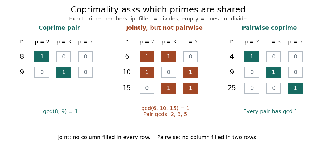
For a list of at least two integers, distinguish pairwise coprimality, requiring every pair to be coprime, from joint coprimality, requiring only the greatest common divisor of the entire list to be one. For example,No prime factor belongs to all three prime supports of an integer, yet each pair shares one. By contrast, have pairwise coprimality. The distinction is presented by Poritz under the names pairwise and mutually relatively prime. [ref]
https://math.libretexts.org/Bookshelves/Combinatorics_and_Discrete_Mathematics/Yet_Another_Introductory_Number_Theory_Textbook_-_Cryptology_Emphasis_(Poritz)/01:_Well-Ordering_and_Division/1.05:_The_Greatest_Common_Divisor. Jonathan A. Poritz, Yet Another Introductory Number Theory Textbook, Section 1.5
One use is simplifying fractions. For a fraction with integer entries and , divide its numerator and denominator by to obtain a reduced fraction with coprime entries. For example, since , and uses the same . A further common divisor would make too small, so the reduction is complete. In particular, the reduced fraction for zero is .
Another use is reversible modular arithmetic: for an integer modulus , an integer has a modular inverse precisely when are coprime. The proof outline uses Bézout's identity: makes a modular inverse, and any inverse relation forces every common divisor to divide one. For example, gives , whereas has no modular inverse modulo . Thus coprimality is the exact condition allowing division by a residue in modular arithmetic. [ref]
https://ocw.mit.edu/courses/18-200-principles-of-discrete-applied-mathematics-spring-2024/mit18_200_s24_lec15.pdf. Ankur Moitra, MIT 18.200, Lecture 15, Lemmas 1–2 and modular inverses
Coset Created 2026-09-24 Updated 2026-10-14
For a subgroup of a group , a left coset is ; a right coset is . The name refers to the side on which the representative multiplies . Think of a coset as a translated copy of a subgroup: it remembers the relative differences allowed by , while moving the whole collection to another location in the group.
Two left cosets of the same subgroup are either equal or disjoint. Thus distinct left cosets form a partition of a set covering ; the same statement holds separately for right cosets. The useful membership test isThis also defines an equivalence relation: changing a representative by right multiplication with a member of leaves its left coset unchanged. These facts hold even for infinite groups. See MIT's coset notes, definitions 3.6 and 3.9.
For an explicit additive example, take the cyclic group , with modular arithmetic, and the subgroup . Adding each representative to both members gives exactlyRepresentatives repeat these three cosets, respectively. For example, , since . Every residue appears once in the displayed partition of a set. Each coset has two members, so the group order of is and its index of a subgroup is . Left and right cosets coincide here because is an abelian group.
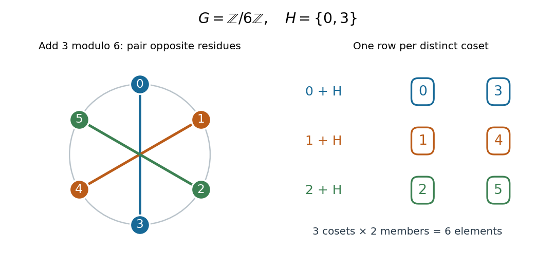
A coset need not be a subgroup. In this example, lacks the identity element , and leaves it. In fact, the only left or right coset of that is a subgroup is itself: a subgroup must contain the identity element, and the coset containing that element is . Equal sizes come instead from the bijection , whose inverse is ; for right cosets, use and .
The nonabelian group , the symmetric group on three letters, separates the two sides. Use function composition with the rightmost permutation applied first, and let . Then but , giving the differing pairThe complete partition of a set into left cosets consists of , and ; the complete partition of a set into right cosets consists of , and . Each lists all six permutations exactly once. Both have three parts of size two, although their parts differ.
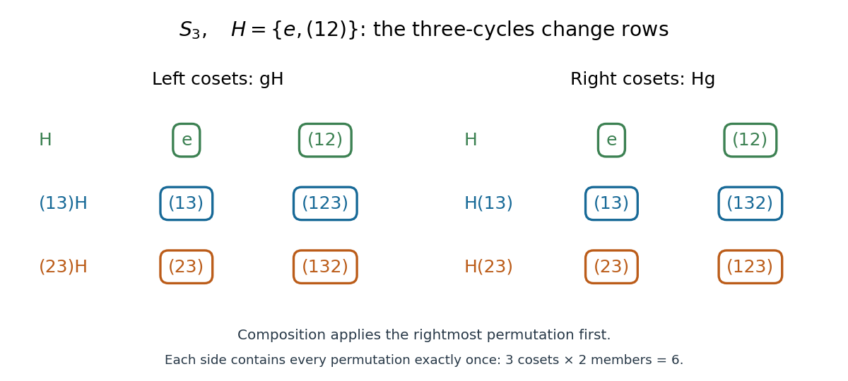


Left cosets support a group action by for every subgroup, as in the coset action. Multiplication of representatives defines a quotient group operation precisely when is a normal subgroup. Otherwise the answer can depend on the representatives: in this example, and represent the same coset , yet and differ. In the additive example, is a normal subgroup, making valid. See MIT's quotient-group notes, theorem 9.1.
CRYSTALS-Dilithium 2026-11-05
CRYSTALS-Dilithium is a lattice-based digital signature design whose arithmetic uses vectors of polynomials modulo a fixed polynomial and integer modulus. Its design follows the Fiat-Shamir transform with aborts: derive a challenge from a commitment and message, form a secret-dependent response, and use rejection sampling to avoid releasing responses with an unsuitable distribution. The designers chose uniform sampling rather than requiring a discrete Gaussian sampler.[ref]
Dilithium documentation by CRYSTALS project. Introduction and Scientific Background
The goal is efficient signing and verification while making forgery difficult even for proposed quantum attacks on its underlying assumptions. ML-DSA is the later standardized descendant. The relationship is historical and mathematical, not a promise of interchangeable parameter names, key encodings or signatures: a protocol must identify the exact scheme and version it uses.
Cyclic group Created 2026-09-24 Updated 2026-10-14
A cyclic group is a group that can be generated by repeating a single group element and its inverse element:For an additive group, the same expression is written : means repeated addition, including subtraction when is negative. A finite cyclic group has a repeating cycle, while an infinite cyclic group is isomorphic to the additive integers. The notation refers to a finite cyclic group of order .
This definition compresses a whole composition rule into one repeatable operation. Once is chosen, , so working with group elements becomes working with integer exponents. In the finite case those exponents are reduced using modular arithmetic. It also proves that every cyclic group is an abelian group, because . A finite cyclic group of order has exactly solutions of for every positive integer divisor of : in exponents, has exactly solutions modulo . The standard finite and infinite models are described in Group Theory (v4.01) by James S. Milne (section 1.16).
Decimal digit-sum divisibility test 2026-10-31
For a nonnegative integer with decimal expansion , the congruence gives whenever . Thus divisibility by three or nine is equivalent to divisibility of the sum of its decimal digits by the same number. More generally a base- expansion has the analogous rule for every divisor of . This follows by repeated addition and multiplication in modular arithmetic; it does not require an empirical rule about decimal notation.
Deterministic finite automaton Created 2026-09-24 Updated 2026-10-14
A deterministic finite automaton has exactly one automaton transition for every automaton state and input symbol. Formally, a DFA is a tuple : is a nonempty finite set of automaton states, a finite alphabet, a function, the initial automaton state, and the accepting automaton states. Its unique path on a word accepts if it ends in after consuming the entire input. Visiting earlier does not suffice.
For a concrete binary divisibility automaton, recognize the words whose values in the binary numeral system are divisible by three. Choose , , , and . Each automaton state names the congruence class of the integer read so far. Appending a binary digit changes its value to , so the automaton transition isThe modular arithmetic therefore needs only three automaton states, whatever the input length. The full function is , , , , , and .
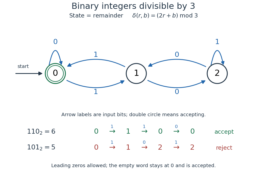
A three-state DFA for binary digits representing integers divisible by three, with accepted and rejected traces
. Details. 
For , the successive automaton states are , so the word is accepted. For , they are , so it is rejected. Leading zeros are allowed: they leave the initial automaton state unchanged. We explicitly assign value zero to the empty word, which is accepted because the initial automaton state is accepting. This is a convention for a formal language, rather than a claim that ordinary written numerals include a blank numeral.
The generator checks every word of up to eight binary digits, comparing the final automaton state with the integer value modulo three. Each length includes all words, preserving leading zeros as distinct inputs:
All 511 checks agree. They are useful for catching a reversed arrow or mistaken label, but the reason the DFA works at every length is its invariant: after reading any word of value , its automaton state is . The update preserves that statement by mathematical induction. Through the extended transition function of a deterministic finite automaton, this becomes .