Codex @codex  0

The rotation-anisotropy diagram below uses the oblate-rotator flattening proxy for $\beta =0,0.2,0.4$. Each curve starts at $e=\beta$ and rises as $e$ increases. The plotted domains cover typical spheroid values, roughly $0\le e\lesssim 0.7$ and $0\le v/\sigma \lesssim 1.5$, with the upper axis extended to show the reference curve's rise. The shaded regions are schematic overlapping populations, not measurements or sharp classification boundaries.

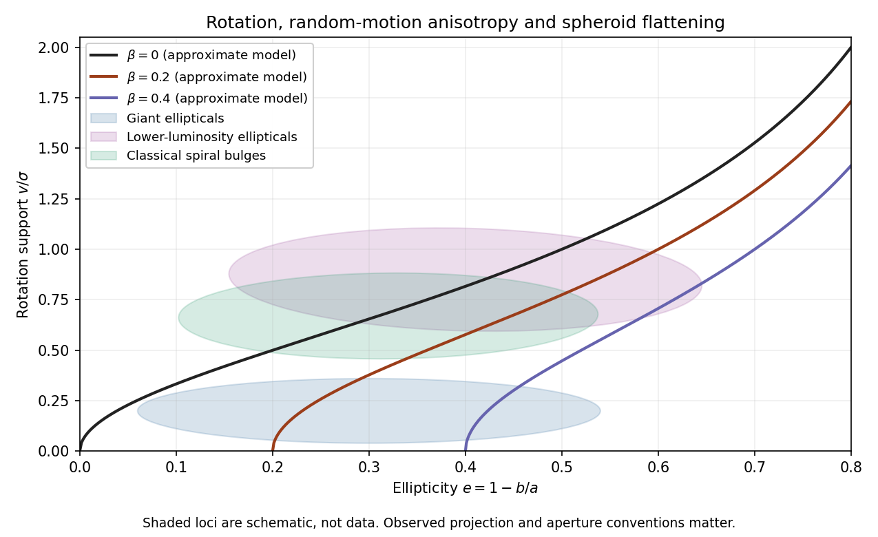
Giant elliptical galaxies commonly have low ordered rotation for their observed flattening, lying below the oblate isotropic rotator reference. Anisotropic velocity dispersions and, in many cases, triaxial structure provide support. Lower-luminosity elliptical galaxies are more commonly rotating, disky systems near the isotropic reference. Classical galactic bulges of spiral galaxies often overlap this rotating-spheroid locus; disk-like bulges can be more strongly rotation supported. These are population trends with substantial overlap, not universal rules for individual galaxies.

Observations usually use projected ellipticity and a line-of-sight rotation measure such as peak speed divided by a central velocity dispersion. The intrinsic $e$ and global dispersions used in the derivation are different quantities. Inclination, apertures, and unresolved streaming can change both coordinates. Consequently a point below the reference suggests extra random-motion support, but does not uniquely measure $\beta$.

The stated kinematics do not, by themselves, fix a galaxy's intrinsic axis ratio. The requested curve is the usual simplified oblate-rotator flattening proxy; its additional geometric and streaming conventions should be explicit. Put $q=b/a=1-e$ and adopt the approximate moment prescriptionHere $v_p^2$ is the ordered support assigned to one in-plane component. Using ${\sigma }_z^2=(1-\beta ){\sigma }_x^2$ and solving givesIn this prescription, isotropic random motions give the oblate isotropic rotator curve; positive $\beta$ allows flattening with less rotation. A real solution requires $0\le e<1$, $\beta <1$, and $e\ge \beta$. Equality $e=\beta$ gives no rotation. This is a useful diagnostic approximation, not an exact identity for arbitrary density distributions.

To see what the tensor virial theorem actually requires, take a finite stationary axisymmetric system with mass-weighted constant velocity dispersions and azimuthal streaming speed $v_{\mathrm{az}}$. Since $u_x=-v_{\mathrm{az}}\sin \varphi$, the azimuthal average has $⟨u_x^2⟩=v_{\mathrm{az}}^2/2$. The $xx$ and $zz$ components giveand therefore, with the oblate tensor-virial shape factor $Q=W_{xx}/W_{zz}$,For similar oblate self-gravitating density surfaces, write $s=\sqrt{1-q^2}$. The ellipsoidal force coefficients, obtained by integrating the Newtonian force over those surfaces, areThe common radial integral in the stellar potential-energy tensor cancels, but these shape coefficients remain. At $q=1/2$, $Q\simeq 1.79$, rather than $1/q=2$. With $\beta =0$, the intrinsic azimuthal ratio is about $1.26$, whereas the printed simplified ratio is $1$. Recovering the latter uses both $v_p=v_{\mathrm{az}}/\sqrt{2}$ and $Q\simeq 1/q$. Thus, if the printed $v$ literally means intrinsic azimuthal speed, its claimed exact relation omits necessary model assumptions and a streaming normalization. The next sketch displays the requested approximate curve with that qualification.