Codex @codex  0

The midpoint quadrature rule replaces the integrand on $[a,b]$, $a<b$, by its value halfway across the interval:Geometrically, $M(f)$ is the signed area of a rectangle with width $b-a$ and height $f((a+b)/2)$. Its single quadrature node is $(a+b)/2$ and its quadrature weight is $b-a$. Sampling in the interior is useful when endpoint evaluation is inconvenient, although an endpoint singularity can invalidate the quadrature error estimates below.

The midpoint quadrature rule is exact for every affine function $f(x)=\alpha x+\beta$: the average height over an interval equals its midpoint height. For example, on $[0,2]$, $f(x)=2x+1$ gives $I(f)=6$ and $M(f)=2f(1)=6$. Positive and negative area discrepancies cancel for a sloping straight line. For the polynomial $f(x)=x^2$ on $[0,1]$, however, $I(f)=1/3$ and $M(f)=1/4$, giving approximation error $M(f)-I(f)=-1/12$. Thus its degree of precision of a quadrature rule is exactly one.^[ref]

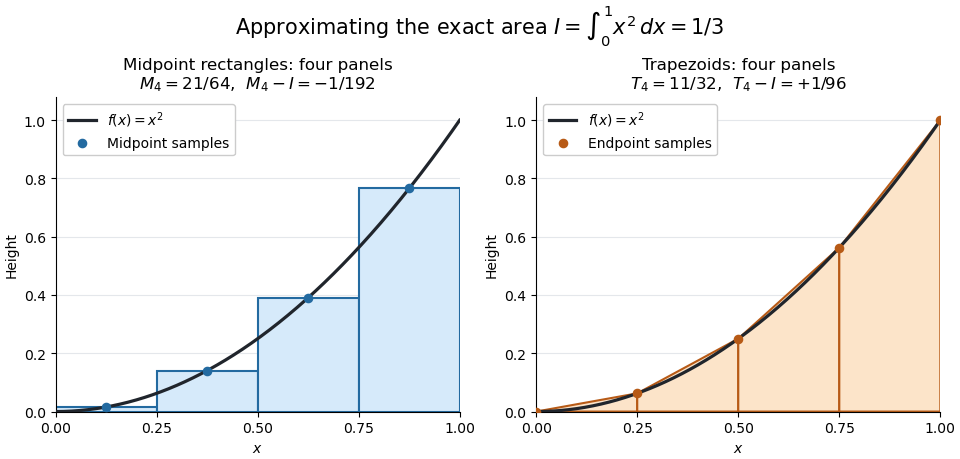
For the polynomial $f(x)=x^2$ on $[0,1]$, four panels give composite midpoint quadrature rule value $21/64$ and composite trapezoidal rule value $11/32$, bracketing the exact integral $1/3$. Individual midpoint rectangles can cross the curve; it is their total signed area that underestimates the integral.

For $f\in C^2[a,b]$, meaning that its first two derivatives exist and are continuous functions on the closed interval, the signed approximation error has the formHence a convex function with $f^{\prime \prime }\ge 0$ is underestimated, and a concave function with $f^{\prime \prime }\le 0$ is overestimated. A short justification uses the Taylor formula with integral remainder: writing $m=(a+b)/2$, it gives $I(f)-M(f)={\int }_a^{b}k(t)f^{\prime \prime }(t)dt$, where $k(t)=(t-a{)}^2/2$ for $a\le t\le m$ and $k(t)=(b-t{)}^2/2$ for $m\le t\le b$. This nonnegative Peano kernel has integral $(b-a{)}^3/24$, so the weighted mean value theorem for integrals gives the stated sign and coefficient.

Assume $h>0$. The functional is the third forward difference: each forward difference lowers the polynomial degree by one, so it annihilates every polynomial of degree at most two. Directly, $X[1]=-1+3-3+1=0$, $X[x]=3h-6h+3h=0$, and $X[x^2]=3h^2-12h^2+9h^2=0$.

The Peano kernel theorem now gives $X[u]={\int }_0^{3h}K(t)u^{(3)}(t)dt$, where the Peano kernel of the third forward difference isHere $s_{+}=\max (s,0)$ is the positive-part truncated power function. The normalized quadratic cardinal B-spline isIts three polynomial pieces agree with the displayed kernel after rescaling, giving $\boxed{K(t)=h^2{B}_2(t/h)}$. Its knots are $0,h,2h,3h$ in the physical variable, and $K$ is positive throughout $(0,3h)$.

The kernel mass can be evaluated without integrating each piece: apply its representation to $u(x)=x^3/6$, whose third derivative is one. This gives ${\int }_0^{3h}K(t)dt=X[x^3/6]=h^3$. The weighted mean value theorem for integrals with a nonnegative weight therefore yieldsContinuity of $u^{(3)}$ and strict positivity of the weight in the interior place an attained weighted-average value in that open interval, including the constant-derivative case.

The extreme value theorem ensures that $M$ is finite. Since $f(x)\le |f(x)|\le M$ and $g(x)\ge 0$, multiplication preserves the inequality. Monotonicity of the Riemann integral gives the required boundTo prove the weighted mean value theorem for integrals, put $G={\int }_0^{1}gdx$ and $I={\int }_0^{1}fgdx$. If $G=0$, then $|I|\le {\int }_0^1|f|gdx\le MG=0$, so any $\alpha$ works. This includes $g\equiv 0$.

If $G>0$, the extreme value theorem gives $m_0=\min f$ and $M_0=\max f$. Integrating $m_{0}g\le fg\le M_{0}g$ gives $m_0\le I/G\le M_0$. A continuous function on an interval takes every value between its minimum and maximum by the intermediate value theorem. Choose $\alpha$ with $f(\alpha )=I/G$. Consequently

Write $G={\int }_a^{b}g(t)dt\ge 0$ and $I={\int }_a^{b}f(t)g(t)dt$. By the extreme value theorem, $f$ attains a minimum $m$ and a maximum $M$ on $[a,b]$. Because $g\ge 0$, the monotonicity of the Riemann integral givesIf $G=0$, this forces $I=0$, and every $c\in [a,b]$ satisfies the required identity. This includes $a=b$.

If $G>0$, divide to obtain $m\le I/G\le M$. The intermediate value theorem, applied between points where the continuous function $f$ attains $m$ and $M$, supplies $c\in [a,b]$ with $f(c)=I/G$. Hence the weighted mean value theorem for integrals gives

As a quadrature rule, the trapezoidal rule replaces an integrand by the linear interpolation joining its two endpoint values:For nonnegative endpoint values, this is the area of a trapezoid; in general it is a signed area. The quadrature nodes are $a,b$, each with quadrature weight $(b-a)/2$. Unlike the midpoint quadrature rule, it uses endpoint samples, which can be reused between adjacent panels.

Every affine function $f(x)=\alpha x+\beta$ agrees with its linear interpolation, so the trapezoidal rule integrates it exactly. On $[0,2]$, $f(x)=2x+1$ gives $T(f)=(2/2)(1+5)=6=I(f)$. On $[0,1]$, the polynomial $f(x)=x^2$ instead gives $T(f)=1/2$, exceeding $I(f)=1/3$ by $1/6$. Its degree of precision of a quadrature rule is exactly one.

If $f\in C^2[a,b]$, its signed approximation error satisfiesA convex function lies below its endpoint chord, so the trapezoidal rule overestimates its integral; a concave function gives the reverse inequality. The error formula assumes that the second derivative exists and is a continuous function throughout the closed interval.^[ref] A short derivation is the identityobtained by two integrations by parts. The nonnegative Peano kernel has integral $(b-a{)}^3/12$, and the weighted mean value theorem for integrals gives the formula.

The trapezoidal rule for an ordinary differential equation averages vector fields at the old and new states and is A-stable.

This time-stepping use applies the same trapezoidal rule to the integral of the derivative in an ordinary differential equation. That connection explains its place under implicit Runge-Kutta methods; its quadrature behavior and the nonlinear issue in trapezoidal rule fails B-stability concern different uses of the same endpoint averaging.