A continuous function sends sufficiently nearby function inputs to nearby function outputs. For a real-valued function and a point that is an accumulation point of , this meansThe approached value and the assigned value must agree. Continuity on means continuity at every point of the domain of a function. At an endpoint of an interval, only approaches inside that domain of a function count. The epsilon-delta definition of continuity below also applies at an isolated point, where continuity holds automatically.[ref]
Calculus Volume 1, §2.4 Continuity. §2.4, Continuity at a Point: definition; Continuity over an Interval: one-sided endpoint conditions
For the polynomial function , approaching makes the function output approach . The continuity bounds for the square function turn this observation into an explicit guarantee: implies . This is useful whenever a small error in an function input must produce a controlled error in an function output. The required input tolerance can depend on the point and on the chosen output tolerance.
The absolute value function is also a continuous function, including at zero: . But its left and right derivatives there are and , so it is not a differentiable function at zero. Continuity controls values without requiring a tangent line. Conversely, a differentiable function is continuous wherever it is differentiable: if , the difference tends to zero with .
Several useful consequences reuse this one local idea. Addition, multiplication and function composition preserve continuity; a quotient of functions is continuous where its denominator is nonzero. On an interval, the intermediate value theorem turns continuity into a guarantee that no intermediate function output is skipped. On a compact set, the extreme value theorem guarantees attained maximum and minimum values. Those extra hypotheses matter: continuity alone on an unbounded domain of a function does not provide a global bound or an attained global maximum.
A rational function such as is continuous on its domain of a function . Zero is excluded from that domain of a function; the missing point prevents a continuous extension there, but it does not make the existing map discontinuous at one of its actual inputs. Always state the domain of a function before judging continuity.
Continuous real-valued functions on a space with a countable dense subset are determined by their restrictions to that subset. The equality set of two such functions is closed and contains the dense subset. Hence there are at most such functions. If the domain is nonempty, distinct constant functions give the matching lower bound.
The set of continuous functions has cardinality . Constant functions provide the lower bound. Restriction to the dense set is injective, since continuity determines a function from its values there. Real sequences have cardinality , by encoding a sequence using its countably many rational lower cuts. Restriction therefore supplies the upper bound and Cantor-Schröder-Bernstein gives equality.
For a continuous function , its zero set is . It is closed and is a G-delta set, since . Replacing by gives the same zero set with values in . In a normal topological space, every closed G-delta set has this form.
A continuous extension of a function to a larger domain is a continuous function satisfying for . The domain and codomain carry specified topologies. Prescribing values on a dense subset does not by itself prove the existence of a continuous extension.
A point of the domain at which a function fails to be continuous. Every discontinuity of a cumulative distribution function is a positive jump, and there are at most countably many: for each positive integer , at most jumps can have size at least .
A point at which a function is continuous. For a real cumulative distribution function , this is equivalent to the associated probability distribution having no atom of a measure at .
A function is continuous at whenFirst choose the required output tolerance ; then choose an input tolerance that works for every allowed function input in that window. Picking a different separately after seeing each would reverse the quantifiers and lose this guarantee. There is no need to exclude , because the output difference is then zero.
At an isolated point of the domain of a function, choose a small enough window that its only allowed function input is . This proves continuity there directly. At a point with arbitrarily close other inputs, the same definition is the limit of a function condition . For metric spaces, replace the two absolute values by their distance functions; for arbitrary topological spaces, the corresponding definition is a continuous map.
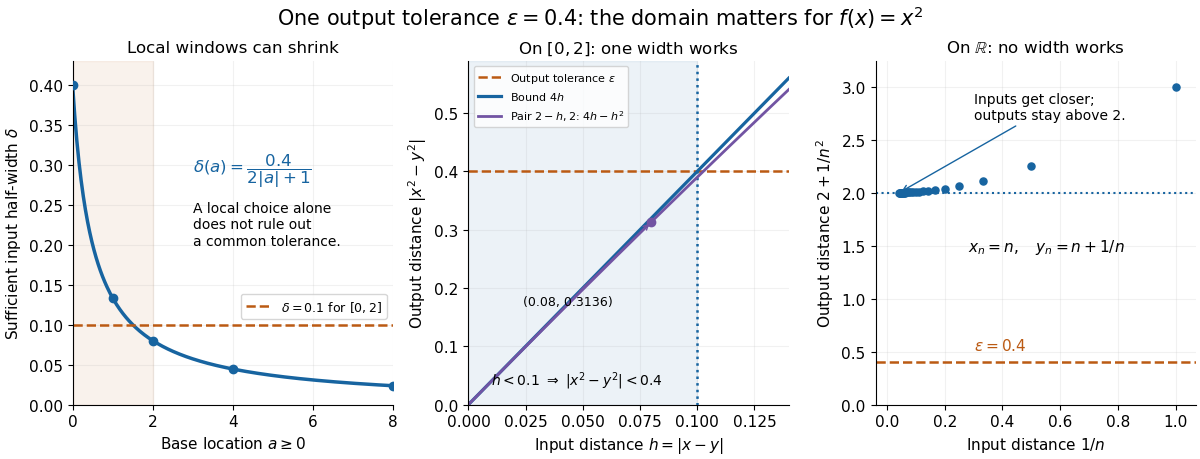
The input tolerance may depend on . A single choice valid everywhere on the domain of a function is the stronger requirement of uniform continuity. The continuous function on shows the difference: for any proposed , the points and have , yet . Thus the fixed output tolerance admits no global input tolerance on the real line.
For at any real , polynomial factorization givesIf , the triangle inequality yields . Therefore the displayed choice of makes imply . This proves continuity and gives an explicit local error bound, rather than an inference from a drawing.
At and , this sufficient choice is . The permitted function inputs satisfy ; their actual function outputs lie in , inside the requested band . A sufficient input window need not be the largest possible one.
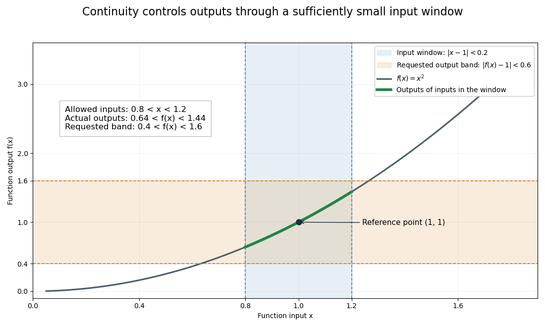
For and , continuity at is equivalent to the following condition: every sequence in with satisfies . This is useful when a numerical method or a proof approaches a point through successively refined function inputs: applying a continuous function preserves the intended limit.
For the forward direction, choose from the epsilon-delta definition of continuity. A convergent sequence eventually lies in that input window, so its function outputs eventually lie in the requested output band. Conversely, if continuity fails, there is some for which every input window contains an allowed with . Choosing such an within of gives while does not tend to . This converse relies on the countable shrinking windows available in metric spaces; a general topological space needs a different formulation.
The Takagi function is a continuous nowhere differentiable function. The triangular summands are continuous and the geometric tail is bounded uniformly. On dyadic intervals of length , all terms of index at least vanish at both endpoints, while every lower summand has slope or . Each refinement therefore changes the secant slope by exactly one in absolute value. The secants straddling a differentiability point lemma rules out a derivative at every real point.
Bounded continuous functions on a topological space form a Banach space with the supremum norm. A uniform limit is continuous and bounded, proving completeness. This space differs from the bounded uniformly continuous functions: free-transport composition is jointly continuous in time and position, but need not be continuous in the global sup norm as time varies.
A real or extended-real function is upper semicontinuous when every strict sublevel set is open. Equivalently its negative is lower semicontinuous. An arbitrary infimum of continuous functions is upper semicontinuous, even when the infimum is over an uncountable family; its strict sublevel sets are unions of the corresponding open sublevel sets.
If near and as , then by the squeeze theorem, even if has no limit. Defining the product to be zero at gives continuity there. For example, extends continuously at zero; the same oscillation near a nonzero multiple of has nonvanishing amplitude and does not have a continuous zero extension.
A function is lower semicontinuous when its strict superlevel sets are open, equivalently when its sublevel sets are closed. In Euclidean spaces this is the sequential lower semicontinuity condition whenever . This closedness property is essential to existence of proximal minimizers.
A function is discontinuous at a point in its domain of a function when it fails the epsilon-delta definition of continuity there. Two basic failures are an incorrect assigned value and unequal one-sided limits. They demand different repairs.
For a removable discontinuity, considerThe limit at zero is , but . Replacing that one value by gives the continuous square function. The sequence makes the mismatch visible: . A removable discontinuity can also describe an expression with a missing value, in which case the question is whether a continuous extension to the missing input exists.
For a jump discontinuity, take for and for . The left and right one-sided limits at zero are and . No assignment to can equal both, so changing only the point value cannot make the function continuous there. Contrast both examples with the corner of : that function is continuous at zero even though its derivative is absent.
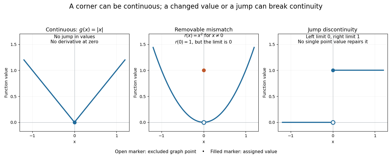
A removable discontinuity has an existing finite limit that differs from the assigned point value, or a missing point value. Changing the point value removes it. Integrals and Fourier coefficients do not detect changes on a set of measure zero, so purely integral hypotheses cannot prohibit this kind of discontinuity for an arbitrary representative.
A jump occurs when both finite one-sided limits of a function exist but differ. Unlike an isolated change in value, a jump changes limiting values on whole one-sided neighbourhoods. One-sided Fourier spectrum excludes jumps explains an obstruction to jumps for functions with only nonnegative Fourier coefficients.
A sublevel set consists of points whose objective value is at most a chosen threshold. Coercivity makes finite sublevel sets bounded, while sequential lower semicontinuity makes them sequentially closed sets in the selected topology.
On a metric space, a functional is sequentially lower semicontinuous exactly when every sublevel set is closed.
A function is locally constant when every point has a neighbourhood on which the function is constant.
The space consists of locally constant complex functions with compact support. On a locally profinite group, finite compact-open coset covers of the support show that every such function is fixed by one common compact-open subgroup under right translation. The symbol infinity describes local constancy in this context, not real differentiability.
The intermediate value theorem says that a real-valued continuous function cannot skip a value between two of its outputs. Let and let be a continuous function on the entire closed interval . ThenThe word "between" includes both endpoint values: choose when , or when . If is strictly between them, every such lies in the open interval . Continuity on means continuity at every interior point, together with the endpoint one-sided limits and . No derivative is required.[ref]
Calculus Volume 1 by Gilbert Strang and others. §2.4, Continuity over an Interval and Theorem 2.11, The Intermediate Value Theorem
For finding a zero of a function, the useful special case isStrictly opposite endpoint signs certify a root bracket, because zero is strictly between and . If an endpoint value is already zero, that endpoint supplies a zero of a function directly; an interior zero of a function need not exist. For example, on has its only zero of a function at the left endpoint. The intermediate value theorem guarantees existence, but neither uniqueness nor a necessary sign-change test. Its numerical usefulness is that the bisection method can turn existence into successively tighter root brackets.
Three explicit functions separate the hypotheses from the conclusion. These are original mathematical illustrations, not measured data.
The polynomial function is a continuous function on , with and . The intermediate value theorem guarantees at least one zero of a function in the interior, while the polynomial factorization displays three: . Thus strict opposite signs do not establish uniqueness.
The everywhere-defined functionhas and , yet no zero of a function. Its jump discontinuity at zero is exactly where the continuity hypothesis fails. A drawn vertical connector would be misleading: the function graph contains neither the intermediate heights nor a zero of a function at that jump. Even continuity only on the interior is insufficient: setting for and gives opposite endpoint signs on with no zero of a function, because the left one-sided limit at is not .
The polynomial function on is a continuous function, and , yet . Its root of a polynomial at zero has multiplicity of a root two. The function graph touches its horizontal tangent line there and stays positive on both sides: existence of a zero of a function does not require a sign change. More generally, near a real root of a polynomial , a polynomial factorization with and has the same sign on both sides sufficiently close to , since the continuous function retains its sign. The intermediate value theorem does not rule out values outside the range between endpoint outputs.[ref]
Calculus Volume 1 by Gilbert Strang and others. §2.4, Example 2.37: positive endpoint values do not exclude an interior zero; Theorem 2.11 requires continuity on the whole interval
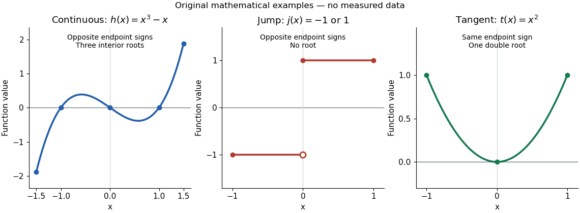
Intermediate value hypotheses: three continuous roots, a jump with no root, and a double root without a sign change
. Details. Consider the original worked example on . First, existence: a polynomial function is a continuous function, and . The intermediate value theorem therefore supplies a zero of a function , even before its value has been calculated.
Second, uniqueness is a separate argument. The derivative is . The derivative criterion for monotonicity, obtained from the mean value theorem, makes a strictly increasing function. Two distinct zeros of a function would contradict that strict increase. Thus this root bracket contains exactly one zero of a function; indeed the same derivative argument proves uniqueness on the entire real line.
Third, localization uses the existing bisection method. Set ; after completed halvings, retain with opposite endpoint signs. Each update tests the old midpoint . The first five exact updates areEvery retained root bracket contains by the intermediate value theorem. After ten halvings, exact arithmetic givesHence . The new midpoint and its bisection error bound areThis midpoint is the estimate after the tenth update; the last tested point was . In general the retained width is , so the bisection error bound is . Nine halvings already suffice for an error at most , since . This guarantee comes from the width of the root bracket, independently of any displayed decimal approximation to the unknown zero of a function. Endpoint signs must be established reliably if evaluations use floating-point arithmetic.
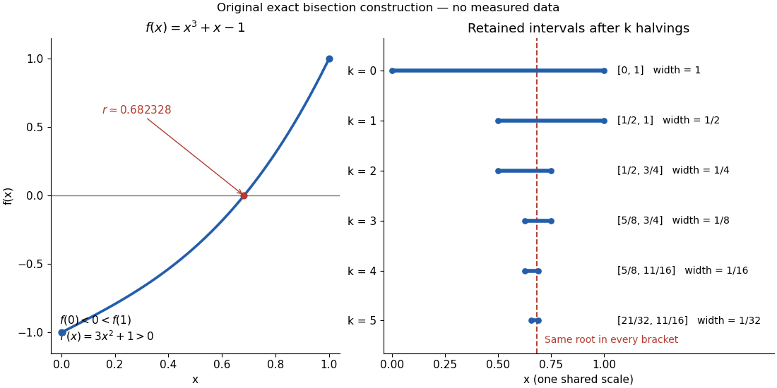
For a short proof outline, endpoint values give the non-strict cases immediately. If is strictly between and , apply the bisection method to the continuous function . A midpoint with finishes the proof. Otherwise retain nested intervals with strictly opposite signs and widths . The nested interval theorem, using completeness of the real numbers, gives a common point to which both endpoint sequences converge. After reversing the sign of if necessary, . Continuity makes both endpoint value sequences converge to , forcing and , hence . The original endpoint values differ from , so . This proof explains why a jump can defeat the construction: shrinking a candidate closed interval cannot supply the missing continuity.
A continuous function on any real interval has image a real interval. Given two image values and an intermediate value, choose preimages and apply the intermediate value theorem on the closed segment joining them, which stays inside the domain. Neither compactness nor boundedness of the original interval is needed. In particular on is a continuous surjection onto : its values are unbounded above and below, so its interval image contains every real number.
A continuous injective real-valued function on a real interval is strictly monotone. A value outside the interval between two endpoint values would, by the intermediate value theorem, create a repeated value. Applying this observation to subintervals gives consistent strict ordering. If the left endpoint value is smaller than the right endpoint value, the function is strictly increasing; otherwise it is strictly decreasing.
If is continuous and , then for every positive integer there is with . For , the continuous difference satisfies . Either one sampled difference is zero or two have opposite signs; the intermediate value theorem then supplies a zero between them. For , the endpoint chord suffices.
If a continuous real-valued function on a real or complex vector space has opposite signs at two points, restricting it to the line segment between them and applying the intermediate value theorem gives a zero.
Every continuous injective function from a real interval to the real line is strictly monotone. A continuous bijection therefore has a continuous inverse.
If is continuous at and is continuous at , then is continuous at .
The continuity set of a function is the set of points where it is continuous. For a real function , define its oscillation at byThe sets are open, and is continuous at exactly when . Hence its continuity set is the Borel set
Two-sided continuity requires both the right and left limits to equal the function value.
A càdlàg function is right-continuous and has a finite left limit at every positive time. The name abbreviates the French phrase /continue à droite, limites à gauche/.
A uniformly continuous function has one input tolerance valid throughout its domain of a function. For , with , uniform continuity meansChoose the output tolerance first, then a positive valid for every pair of function inputs. It may depend on , the function and its domain of a function, but not on the pair’s location. The absolute values measure input and output distance.[ref]
Basic Analysis: Introduction to Real Analysis, Volume I by Jiří Lebl. §3.4, Definition 3.4.1: a single positive input tolerance for all pairs in the specified real domain
Compare the quantifier order with the epsilon-delta definition of continuity:Both lines end with . In the first, can depend on the point ; in the second, it is chosen before . Thus uniform continuity implies continuity at every point. Each requested gets its own shared tolerance.
For an exact example, take the polynomial function on the closed interval . For every pair of function inputs in that interval, polynomial factorization givesConsequently works everywhere on this domain of a function. With , the common tolerance is . Near the right endpoint, for example, and have input distance and output distance . The bound is sufficient; it does not claim the largest admissible input window at each point.
On the whole real line, the same polynomial function is a continuous function but fails uniform continuity. Take the sequences and , for positive integers . ThenFor any proposed , choose an integer . The inputs are closer than , yet their outputs violate the fixed tolerance . The sequences need not themselves have a finite limit: their mutual distance is what tends to zero. This is the obstruction captured by the sequential criterion for uniform continuity. Restricting the domain of a function to removes these escaping pairs.
A uniformly continuous function need not be a bounded function. The identity function on the real line has , so always works, although its image of a function is the unbounded real line. Uniform continuity controls changes between nearby inputs, not the overall size of outputs. Likewise, an unbounded domain of a function does not by itself prevent uniform continuity.
The square root supplies a different common tolerance on the interval . Assuming , put and . Since ,Interchanging the inputs when necessary provesThus guarantees uniform continuity on the entire domain of a function, including zero. For , any input distance below suffices. The pairs and both have input distance ; their output distances are respectively and . The common guarantee accommodates quite different local sensitivities.
This Hölder continuity bound allows a curved tolerance rule. It is weaker than a Lipschitz bound: at zero the output change divided by the input change isNo finite Lipschitz constant works near zero, even though uniform continuity does. A Lipschitz function does have uniform continuity, choosing when its Lipschitz bound is positive; when it is a constant function.[ref]
Basic Analysis: Introduction to Real Analysis, Volume I by Jiří Lebl. §3.4, Proposition 3.4.8 and Example 3.4.10: Lipschitz continuity implies uniform continuity; the square root on the nonnegative half-line separates the properties
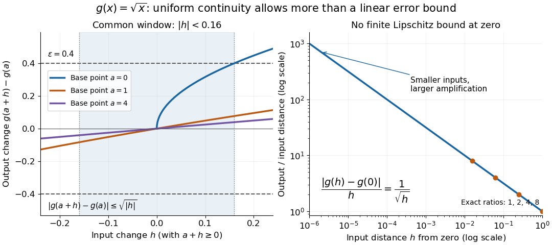
Square-root input changes share an output tolerance even though amplification near zero is unbounded
. At left, the exact output changes for base points stay inside whenever and . The right panel computes the amplification for inputs : it grows without bound as decreases. These are calculated function graphs, with no experimental measurements. Details.For general metric spaces, replace the absolute values by the respective distance functions. The Heine-Cantor theorem gives an existence guarantee: every continuous function on a compact metric space is uniformly continuous. In particular, continuity on a finite closed interval provides a common tolerance, even when no simple formula for it is known.[ref]
Basic Analysis: Introduction to Real Analysis, Volume I by Jiří Lebl. §7.5, Definition 7.5.10 and Theorem 7.5.11: uniform continuity between metric spaces and the compact-domain theorem
For a short proof outline, fix . Continuity gives each point an open ball of radius within which outputs differ from by less than . The open balls of half these radii still cover the domain of a function. Compactness supplies a finite subcover. Take to be the smallest half-radius in this finite set. Two inputs closer than lie together in one of the original open balls, so the triangle inequality bounds their output distance by . The beautiful step is that the compact set turns local choices into finitely many choices, whose minimum stays positive.
A shared tolerance also makes uniformly continuous functions preserve Cauchy sequences: after choosing for , all sufficiently late input pairs are closer than , so all corresponding output pairs are closer than . Unlike a convergent sequence argument, this does not require an input limit inside the domain of a function. It is why uniform continuity is useful for extending a function toward missing endpoints and for the decay argument below.
A nonnegative function that is a uniformly continuous function on the interval and has a finite integral tends to zero. Otherwise uniform continuity gives disjoint intervals of a fixed width on which the function exceeds a fixed positive value, contradicting integrability. This supplies a useful decay argument for Lyapunov functions with merely continuous vector fields.
To make the fixed width explicit, suppose some occurs as a lower bound along a sequence with . Choose from uniform continuity for output tolerance . On every interval lying in , the function is greater than . Extract a subsequence whose centers are more than apart. Each disjoint interval contributes at least to the integral, so the first contribute at least . This contradicts finiteness of the integral. The same input width at every center is the essential step; continuity alone would allow progressively narrower peaks.
Articles by others on the same topic

A continuous function is a type of mathematical function that is intuitively understood to "have no breaks, jumps, or holes" in its graph. More formally, a function \( f \) defined on an interval is continuous at a point \( c \) if the following three conditions are satisfied: 1. **Definition of the function at the point**: The function \( f \) must be defined at \( c \) (i.e., \( f(c) \) exists).



