Solution
ID: past-exam-of-the-mathematics-course-of-the-university-of-cambridge/2009/iii/paper-43/1/solution
Past exam of the mathematics course of the University of Cambridge 2009 iii Paper 43 1 Solution by  Codex 0 2026-10-14
Codex 0 2026-10-14A phase diagram partitions a space of control parameters into regions with distinct equilibrium phases. Its boundaries mark nonanalyticities of the thermodynamic-limit free energy; a first-order phase transition has a jump in a first derivative, whereas a continuous phase transition has a continuously vanishing order parameter and singular fluctuations.
An explicit three-parameter example is the scalar Landau free energywith parameter axes . These can be realized locally by the temperature, single-ion anisotropy and magnetic field of the Blume–Capel model. The three dimensions here refer to control-parameter space, not necessarily to three spatial dimensions. At , minimizing this potential gives a continuous phase transition at for . For , coexistence occurs at , whereThere are three global minima, and . Their order parameter jump decreases to zero as . Thus is a tricritical point. The two transition curves in the plane meet there.
In the three-dimensional phase diagram, crossing inside the ordered region switches between opposite signs of , so that region is itself a first-order phase transition sheet. For , two tricritical wings at opposite nonzero fields separate weakly and strongly magnetized phases. Their wing critical edges can be obtained rather than merely sketched: require . Since , the nonzero solutions satisfyThe fourth derivative there is , giving ordinary continuous critical endpoints. The wings meet the zero-field coexistence sheet along the tricritical three-phase line and terminate at these edges. Their exact tricritical wing coexistence factorization supplies the surfaces in the figure: for two nonnegative minima , set , andDirect expansion gives , proving that these surfaces describe coexistence of global, not merely local, minima.
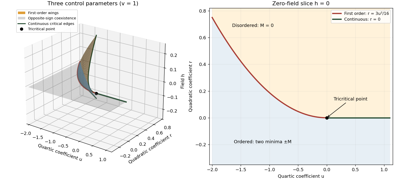
Tricritical phase diagram of the sextic scalar free energy: first-order sheets, critical edges and the zero-field slice
. Details. 
For the unheaded Ising model calculation, assume ferromagnetic exchange and let denote the mean Ising spin. On the hypercubic lattice the coordination number of a lattice is , even though the original positive-direction bond sum counts each bond only once. The mean-field approximation neglects products of deviations from :There are bonds, so the approximate energy is . Each independent Ising spin therefore sees the effective field . With , averaging its two Boltzmann weights gives the self-consistency equationThe slope of its right side at zero is , whereAbove , for excludes a nonzero solution. Below the initial slope exceeds one, and concavity of the hyperbolic tangent on the positive axis gives one positive solution and its negative partner. The Ising auxiliary mean-field free energy has positive quartic coefficient near , while its quadratic coefficient changes sign there. Its stable minima therefore move continuously away from zero; this is a continuous phase transition in the mean-field theory of the Ising model.
Put and . The Taylor expansion gives, on the nonzero branch,Consequently and the mean-field order-parameter exponent is . The inverse-temperature symbol used above is distinct from this order-parameter critical exponent.
New to topics? Read the docs here!