Paul trap secular-motion example
ID: paul-trap-secular-motion-example

Choose these dimensionless parameters for an original example, with no collisions or damping. They are teaching inputs, not measurements from either lecture. With and slow initial amplitude , the radial equation and its leading approximation areSet and to match the approximate initial conditions. The leading secular angular frequency is . The velocity Verlet method integrates the full RF equation over 80 drive periods; a separate fourth-order Runge-Kutta method checks the computed trajectory. Halving the timestep tests numerical error independently of the averaging error.
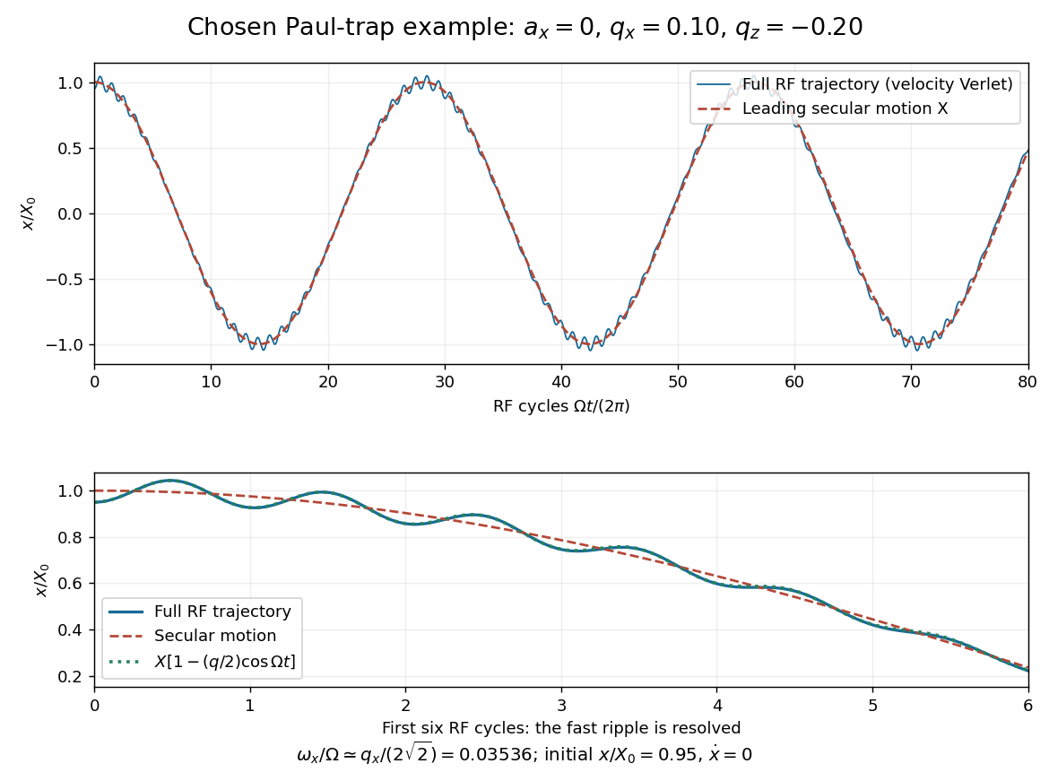
Full RF motion and the leading secular approximation
. Original chosen small-parameter calculation in units of . The lower panel resolves six drive cycles and includes the first micromotion correction. Agreement over this finite interval does not establish a stability diagram or an exact secular frequency. Details.
Using 400, 800, 1600 and 3200 steps per RF period gives successive maximum position differences of approximately , and in units of , consistent with second-order convergence. The finest trajectory differs from the independent classical fourth-order Runge-Kutta method result by at most , whereas differs by as much as . Over a sufficiently long time, the omitted correction to the secular angular frequency produces a growing phase discrepancy even if the numerical trajectory has converged. For the chosen point only, integration of a fundamental solution matrix over one RF period checks that both the radial and axial Floquet multipliers lie on the unit circle, away from its endpoints. This tests simultaneous ideal confinement without extrapolating to larger .
New to topics? Read the docs here!