Codex @codex  0

A Type Ia supernova can be standardized as a standard candle by correcting its peak brightness using the light curve shape and colour index. Its host spectrum gives the redshift; the corrected apparent magnitude and calibrated absolute magnitude give the distance modulusThe resulting Hubble diagram measures the shape of the luminosity distance as a function of redshift. A spatially flat matter-and-vacuum model, for example, predictsNonzero cosmological spatial curvature changes both the expansion rate and the conversion from radial to transverse comoving distance. Comparing the observed Hubble diagram with these predictions constrains the matter density parameter, cosmological constant and cosmological spatial curvature; a single low-redshift observation cannot separate them. The nearby sample calibrates the common intercept, while distant Type Ia supernovae supply the redshift-dependent shape. Relative faintness at a specified redshift means a greater inferred luminosity distance.

Type Ia supernova cosmology requires correction for interstellar extinction, possible evolution of the standardized luminosity, and selection bias. The absolute magnitude–Hubble constant degeneracy means that an uncalibrated sample constrains the shape rather than independently determining $H_0$.

Type Ia supernovae have similar peak luminosities that can be standardized using their light-curve width and color, rather than assumed to be identical without correction. Their redshifts and corrected apparent magnitudes give a distance modulus,Compare this Hubble diagram with the luminosity-distance prediction of a background cosmology. Restoring $c$, put $E(z)=H(z)/H_0$, $I(z)={\int }_0^{z}d{z}^{\prime }/E(z^{\prime })$ and define ${\mathcal{S}}_{{\Omega }_k}(I)$ as $\sinh (\sqrt{{\Omega }_k}I)/\sqrt{{\Omega }_k}$ for ${\Omega }_k>0$, $I$ for ${\Omega }_k=0$, and $\sin (\sqrt{-{\Omega }_k}I)/\sqrt{-{\Omega }_k}$ for ${\Omega }_k<0$. ThenNeglecting radiation at these redshifts, Friedmann equations and a separately conserved dark energy component with $w(z)=p/(\rho c^2)$ giveFor constant $w$, the last factor is $(1+z{)}^{3(1+w)}$; a cosmological constant has $w=-1$. Thus the redshift dependence of the measured distance constrains matter density, curvature and the dark-energy equation of state. At small redshift, $d_L=(cz/H_0)[1+(1-q_0)z/2+\cdots ]$, showing how departures from the linear Hubble law probe the deceleration parameter.

The early distant-supernova analyses found larger distances than matter-only decelerating models predicted, providing evidence for accelerated expansion; see the 1998 supernova analysis and the 1999 independent supernova analysis. This is a statement about the distance-redshift curve under the standardization and cosmological assumptions, not a direct measurement of a fluid pressure.

The absolute magnitude–Hubble constant degeneracy means uncalibrated supernovae constrain the shape of $d_L(z)$ without separately determining $H_0$ and the common absolute luminosity. The integral over $H(z)$ also makes different matter, curvature and $w(z)$ histories partly degenerate. Wide redshift coverage and independent cosmic microwave background and large-scale structure of the universe information help break these degeneracies. Dust extinction, source evolution, photometric calibration, sample selection and K corrections must be modeled, and constraints on a time-dependent equation of state depend on how that function is parameterized. Standardized supernovae test the expansion history; they do not by themselves uniquely determine every cosmological parameter.

Choose a fixed $H_{\mathrm{ref}}>0$, and write $h(H_0)=-5{\log }_{10}(H_0/H_{\mathrm{ref}})$ and $d_s(w,{\Omega }_M)=\mu (z_s;H_{\mathrm{ref}},w,{\Omega }_M)$. The predicted magnitude is $M_0+h(H_0)+d_s$. Thus the likelihood depends on $M_0,H_0$ only through $\beta =M_0+h(H_0)$, the absolute magnitude–Hubble constant degeneracy. Since $d{M}_0=d\beta$ at fixed $H_0$, integrating with a flat density over the entire real line removes $H_0$.

Explicitly, let $a_s=(v+r_s{)}^{-1}$, $S={\sum }_s{a}_s$, $x_s={\hat{m}}_s-d_s$, $\bar{x}=S^{-1}{\sum }_s{a}_s{x}_s$ and $Q={\sum }_s{a}_s(x_s-\bar{x}{)}^2$. Completing the square gives ${\sum }_s{a}_s(x_s-\beta {)}^2=Q+S(\beta -\bar{x}{)}^2$, so flat-prior elimination of a Gaussian common mean yieldsindependently of $H_0$. The proportionality includes the arbitrary constant of the flat prior, which cancels within this posterior analysis.

If the remaining posterior integral is finite, prior independence gives $p(H_0\mid \mathcal{D})\propto p(H_0)$ and hence $\boxed{p(H_0\mid \mathcal{D})=p(H_0)}$: these data supply no marginal update of the Hubble constant. The quoted Gaussian is consequently retained with its stated $a,b$. Strictly, the model uses $H_0>0$ inside a logarithm, so the Gaussian prior must be restricted and normalized on that domain:where $\varphi ,\Phi$ are the standard normal density and distribution function. Ignoring its negligible negative tail gives the stated untruncated Gaussian approximation.

Stipulate $H_0=70\mathrm{km}{\mathrm{s}}^{-1}\mathrm{Mp}{\mathrm{c}}^{-1}$ and $c=299792.458\mathrm{km}{\mathrm{s}}^{-1}$, so $c/H_0=4282.7494\mathrm{Mpc}$. A megaparsec is $10^6$ parsecs. Neglect radiation in cosmology. Compare an accelerating flat model $({\Omega }_{m,0},{\Omega }_{\Lambda ,0})=(0.3,0.7)$, an open matter-only model $(0.3,0)$ and the Einstein-de Sitter universe $(1,0)$. Their present deceleration parameters are respectively $-0.55$, $0.15$ and $0.5$. For these models,Here $\chi$ is dimensionless; the radial null geodesic in FLRW spacetime supplies its integral and spatial curvature of an FLRW universe supplies $S_k$. The observer-to-source comoving radial distance is $(c/H_0)\chi$, whereas the transverse distance uses $S_k$. Omitting the latter distinction would bias the open-model comparison.

At $z=0.5$, numerical integration gives $\chi =0.440984335$ for the flat accelerating model and $\chi =0.392227378$ for the open matter-only model. ThusThe accelerating model is $0.21559$ mag fainter than the open matter-only prediction at the same redshift and standardized absolute magnitude, corresponding to $1.10438$ times the luminosity distance and $0.81991$ times the radiative flux. These are model calculations, not observations from either collaboration.

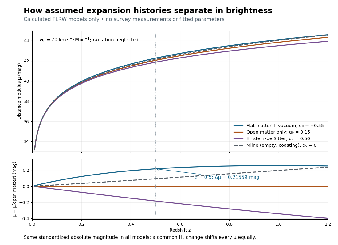
The Milne model has $q=0$, ${\Omega }_{m,0}={\Omega }_{\Lambda ,0}=0$ and ${\Omega }_{k,0}=1$, giving $\chi =\log (1+z)$ and $d_L=(c/H_0)(z+z^2/2)$. The Einstein-de Sitter luminosity-distance relation independently checks the flat matter-only integral. At $z=0.5$, the accelerating model exceeds the Milne model by only $0.12317$ mag, illustrating the dependence of a residual on the chosen reference. Over a longer redshift interval, luminosity distance integrates past deceleration as well as recent acceleration; a residual need not increase forever.

Multiplying $H_0$ by $f>0$ at fixed density fractions divides every $d_L$ by $f$ and shifts every distance modulus by $-5{\log }_{10}f$. The predicted apparent magnitude is unchanged if $M_{B,0}$ simultaneously increases by $5{\log }_{10}f$. This is the absolute magnitude–Hubble constant degeneracy. For example, $70\to 77\mathrm{km}{\mathrm{s}}^{-1}\mathrm{Mp}{\mathrm{c}}^{-1}$ shifts $\mu$ by $-0.20696$ mag and $M_{B,0}$ by $+0.20696$ mag. Relative curves at the same $H_0$ retain their separation; determining $H_0$ requires an external absolute magnitude calibration.