Take independently decaying atomic nuclei, each with lifetime drawn from an exponential distribution of rate . With no replenishment, the survivor count isEach indicator variable has success probability , so the binomial distribution givesThe smooth population law is the expected value , satisfying . One realization instead loses whole atomic nuclei at discrete times. An observed count above the smooth curve need not contradict the mathematical model.
For an original chosen example, let and half-life . Then . After , the survival probability is , givingThe standard deviation describes variation between repeated populations governed by these assumptions. It is not an uncertainty interval for a noiseless deterministic curve.
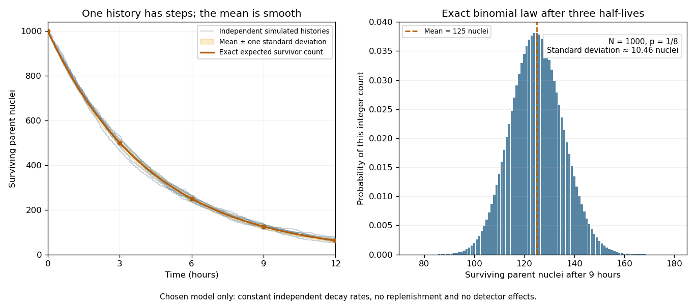
Random survivor counts and the smooth radioactive-decay law
. Original constant-rate model with independent parent atomic nuclei and a half-life. Simulated histories are compared with their exact expected value and a one-standard deviation band. The second panel shows the exact binomial distribution after three half-lives. These are model calculations, not measurements from a historical sample. Details.
Articles by others on the same topic
There are currently no matching articles.