Codex @codex  0

Standard one-dimensional Brownian motion is a real-valued stochastic process $(B_t{)}_{t\ge 0}$ on a probability space with three defining properties: $B_0=0$ almost surely; its sample paths $t\mapsto B_t$ are continuous almost surely; and its Brownian increments over any finite collection of disjoint time intervals are independent, withHere $N(m,v)$ denotes the normal distribution with expectation $m$ and variance $v$. The alternative symbol $W_t$ denotes the same kind of stochastic process. Continuity is a simultaneous statement about an entire sample path, rather than a separate assertion at each fixed time. Relative to its natural Brownian filtration, a future Brownian increment is independent of all observations up to its starting time.

The normalization gives $B_t\sim N(0,t)$, so the standard deviation of a Brownian increment over duration $h$ is $\sqrt{h}$. For $h=1$, $0.01$, and $0.0001$, the corresponding standard deviations are $1$, $0.1$, and $0.01$. Time becoming one hundred times shorter makes typical displacement ten times smaller. Brownian scaling expresses this rule for the whole stochastic process, while the Brownian covariance kernel describes how positions at different times remain related despite independent increments.

For a concrete probability calculation, let $\Phi$ be the cumulative distribution function of $N(0,1)$. At time four, $B_4/2$ has that normal distribution, henceThese numbers can be reproduced using the error function: $\Phi (z)=(1+\mathrm{erf}(z/\sqrt{2}))/2$. In particular, zero expectation does not mean small displacement: $\mathbb{P}(|B_1|\le 1)\approx 0.6826894921$, but the same fixed interval contains only about $38.3\%$ of the probability at time four.

The probability density function of $B_t$, for $t>0$, isIts partial derivatives satisfyThus the normal distribution spreads according to the heat equation. Starting at a fixed position $x_0$ replaces $x$ by $x-x_0$. This is a useful bridge between individual random trajectories and the deterministic evolution of their probability density function: the same Brownian motion provides both descriptions.

Physical diffusion uses its own scale. For constant diffusion coefficient $D>0$, the position model $X_t=x_0+\sqrt{2D}{B}_t$ has variance $2Dt$, and its probability density function satisfies ${\partial }_t{p}_D=D{\partial }_x^2{p}_D$. For example, $D=0.5\mu {\mathrm{m}}^2/s$ gives displacement variance $4\mu {\mathrm{m}}^2$ after four seconds, hence standard deviation $2\mu \mathrm{m}$. Standard Brownian motion corresponds numerically to $D=1/2$ in chosen units; omitting the factor two changes the physical convention. Einstein's 1905 paper relates diffusion to the mean squared displacement in precisely this convention. ^[ref]

Continuity does not supply a smooth physical velocity. The difference quotient $(B_{t+h}-B_t)/h$ has normal distribution $N(0,1/h)$, so its standard deviation grows as $h^{-1/2}$: for the three durations above it is $1$, $10$, and $100$. This calculation motivates the nowhere differentiability of Brownian motion, but it alone is not a proof of the simultaneous assertion at every time. The theorem says that, with probability one, no finite derivative exists anywhere along the sample path. A drawn polygon only displays a finite grid; its straight segments cannot establish this theorem. See Theorem 7.1.6 in Probability: Theory and Examples (fifth edition) by Rick Durrett.

For physical particles, Brownian motion is a model of position on suitable observation scales. It does not claim that microscopic velocity is a derivative of this idealized path. Einstein explicitly restricts his assumption of independent increments to intervals that are not too short. ^[ref]

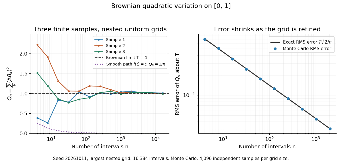
Another way to measure the roughness is quadratic variation. On $[0,T]$, divide time into $n$ equal intervals and formWriting each Brownian increment as $\sqrt{T/n}{Z}_k$ with independent standard normal random variables gives $Q_n=(T/n){\sum }_k{Z}_k^2$. Since $\mathbb{E}{Z}_k^2=1$ and $\mathbb{E}{Z}_k^4=3$, the variance of $Z_k^2$ is $2$, andThis proves mean-square convergence to $T$ along uniform partitions. For $T=2$ and $n=100$, the expectation is $2$, the variance is $0.08$, and the root mean square of the error is $\sqrt{0.08}\approx 0.2828427125$. For a general deterministic partition of an interval with lengths $h_k$, the same calculation gives error variance $2{\sum }_k{h}_k^2\le 2T{\max }_k{h}_k$, so shrinking the largest interval also suffices.

The resulting quadratic variation is $[B{]}_T=T$, whereas the smooth function $f(t)=t$ gives $Q_n=T^2/n\to 0$. This difference explains why the ordinary rules of calculus need the second-order correction in the Itô formula. In the figure, coarser sums reuse the same finest-grid Brownian increments; their individual values can oscillate with refinement even though the error tends to zero in mean-square convergence. Refining a fixed interpolating polygon forever would instead give zero quadratic variation, so the finite-grid illustration must not be confused with the limiting Brownian motion.

Historically, Brown's 1828 report describes microscopic observations made in 1827, starting with particles released from pollen and extending to inorganic materials; this challenged an explanation based solely on living matter. His observations and the later mathematical model are distinct contributions. ^[ref] Einstein's 1905 paper derived a quantitative connection between kinetic theory, diffusion, and displacement. ^[ref] Wiener's 1923 Differential-Space developed integration on spaces of paths, a foundation for Wiener measure; it also acknowledges earlier work and his own previous papers. These dates mark documented contributions rather than an assertion that each subject had a single discoverer. ^[ref]

Let $\tau$ be the first attainment of the maximum of standard Brownian motion on $[0,T]$, with $T>0$. Time reversal shows $\tau <T$ with probability one. Then $Y_t\le 0$ for $0\le t\le T-\tau$, an initial interval of positive length. Standard Brownian motion has probability zero of this property by the Brownian reflection principle, so $Y$ is not Brownian. Moreover $\tau$ is not a stopping time for the natural Brownian filtration: for $0<t<T$, $\mathbb{P}(\tau \le t\mid {\mathcal{F}}_t)=2\Phi ((M_t-B_t)/\sqrt{T-t})-1$, which is strictly between zero and one on $\{B_t<0\}$. The Strong Markov property is therefore inapplicable at this random time.

In a one-factor market whose filtration is the usual augmentation of the natural Brownian filtration, with nonzero spot volatility and local martingale deflator $Y$, the Brownian martingale representation theorem constructs a nonnegative replicating strategy for a bounded nonnegative contingent claim. The minimal initial cost among nonnegative self-financing portfolios is $\mathbb{E}[Y_T{\xi }_T]$.

In the completed natural Brownian filtration, suppose $d{S}_t/S_t={\mu }_{t}dt+{\sigma }_{t}d{W}_t$ with ${\sigma }_t\ne 0$, and let $d{\zeta }_t=-{\zeta }_t(r_{t}dt+{\kappa }_{t}d{W}_t)$, ${\kappa }_t=({\mu }_t-r_t)/{\sigma }_t$. For an affordable nonnegative terminal claim $X$, represent the conditional-expectation martingale $N_t=\mathbb{E}[{\zeta }_{T}X\mid {\mathcal{F}}_t]$ as $d{N}_t=h_{t}d{W}_t$. Then $w_t=N_t/{\zeta }_t$ and the displayed dollar amount in the stock replicate $X$. The Itô product rule gives $d(\zeta w)=\zeta (\sigma \theta -\kappa w)dW$, proving the formula; share holdings are ${\theta }_t/S_t$.

On a probability space $(\Omega ,\mathcal{F},\mathbb{P})$, a standard one-dimensional Brownian motion is a real-valued stochastic process $B=(B_t{)}_{t\ge 0}$ with $B_0=0$ almost surely, continuous sample paths almost surely, and independent increments, such thatHere the second parameter is the variance. Thus its Brownian increments have the normal distribution with mean zero and variance equal to elapsed time. Equivalently, relative to a specified filtration $({\mathcal{F}}_t)$, require $B$ to be an adapted process and $B_t-B_s$ to be independent of ${\mathcal{F}}_s$ with this normal distribution. Taking the natural Brownian filtration recovers the first definition.

Write $e_t=1_{[0,t]}$ as an element of L2 space. Parts (iii) and (iv) show that $B_t=W{e}_t$ is a centered Gaussian process with covariance functionIn particular $B_t-B_s\sim N(0,|t-s|)$. The fourth moment of a centered normal random variable of variance $v$ is $3v^2$, soThe Kolmogorov continuity theorem, with moment exponent $4$ and time exponent $2>1$, provides a continuous modification $\hat{B}$. At each finite set of times this modification of a stochastic process has the same joint law as $B$.

For $0\le t_0<t_1<\cdots <t_m\le 1$, the successive increments are Jointly Gaussian. The covariance of two increments on disjoint intervals equals the inner product of their disjoint interval indicators and is zero. Zero cross-covariances of Jointly Gaussian variables imply independence, and each increment has variance $t_j-t_{j-1}$. Finally $e_0=0$ in L2 space, so ${\hat{B}}_0=0$ almost surely. ThereforeIndependence from the whole past in its natural Brownian filtration follows by extending finite-dimensional independence to the generated sigma-algebra.

Use ${\theta }_t$ for the dollar amount invested in the stock; the number of shares is ${\theta }_t/S_t$. The bank account contains $w_t-{\theta }_t$ dollars. With no intermediate consumption, the self-financing portfolio equation isIf instead $\theta$ denotes share holdings, replace each dollar ${\theta }_t$ here by $S_t{\theta }_t$. The equation says that trading only reallocates existing portfolio wealth; gains come from cash interest and stock returns.

For the standard unconstrained complete-diffusion formulation, assume the completed natural Brownian filtration, initial wealth $w_0>0$, and nonnegative admissible wealth. Define the market price of risk ${\kappa }_t=({\mu }_t-r_t)/{\sigma }_t$. The boundedness assumptions make $\kappa$ bounded. The state-price density normalized at zero isIts money-market-adjusted process $Z_t=e^{{\int }_0^t{r}_{s}ds}{\zeta }_t$ is a true martingale by the Novikov condition. Under $d\mathbb{Q}=Z_{T}d\mathbb{P}$, the Girsanov theorem gives $W_t^{\mathbb{Q}}=W_t+{\int }_0^t{\kappa }_{s}ds$ as a Brownian motion, and the discounted stock has zero drift.

The Itô product rule applied to the wealth equation givesFor nonnegative admissible wealth this is a nonnegative local martingale, hence a supermartingale. Therefore every affordable terminal payoff $X=w_T$ satisfies the state-price budget constraint $\mathbb{E}[{\zeta }_{T}X]\le w_0$. Nonzero volatility and the Brownian martingale representation theorem allow replication of nonnegative claims with finite state-price cost.

For a differentiable strictly concave utility function with the usual conditions ensuring an interior integrable optimizer, put $I=(U^{\prime }{)}^{-1}$, the inverse marginal utility. Pointwise maximization of $U(x)-y{\zeta }_{T}x$ givesThe second equation determines the positive constant $y$. To prove optimality, use the concave supporting-tangent inequality:Taking expectations and using the budget bound proves that the candidate dominates every admissible affordable payoff, whenever the utility expectations are well defined. This is the complete-market terminal utility optimizer.

The actual wealth and dollar portfolio are as explicit as general adapted coefficients permit. LetThe Brownian martingale representation theorem, with localization if only $L^1$ integrability is initially known, gives $h$. The dollar portfolio from a deflated wealth martingale isThe bank holds $w_t^{\ast }-{\theta }_t^{\ast }$ dollars. Equivalently, with $B_t=e^{{\int }_0^t{r}_{s}ds}$, $w_t^{\ast }=B_t{\mathbb{E}}^{\mathbb{Q}}[w_T^{\ast }/B_T\mid {\mathcal{F}}_t]$. These formulas need no unjustified differentiability of a value function with random coefficients.

The printed assumption that $U$ is only increasing and concave does not guarantee that the interior formula exists, or even that the optimal value is finite. In general replace the inverse formula by an affordable selectionwhere $\mathcal{D}$ is the wealth domain; boundary choices or supporting slopes handle nondifferentiability. Existence, finite cost and replication still have to hold. A concrete obstruction is the unbounded linear terminal-wealth utility: take $U(x)=x$, $r=0$, $\mu =\sigma =1$, and the Brownian filtration. Then ${\zeta }_T=e^{-W_T-T/2}$. For $A_n=\{{\zeta }_T<1/n\}$, the bounded nonnegative claimis replicable, costs $w_0$, and has $\mathbb{E}{X}_n>n{w}_0$. Thus there is no finite optimal expected utility under the literal utility hypotheses alone. Also, bounded coefficients do not ensure market completeness in an arbitrarily enlarged filtration containing untraded randomness; the full replication formula uses the Brownian market information assumption stated above.

Assume the usual positive initial asset values. The coefficients determine a unique normalized local martingale deflator. The state-price density and local deflator distinction matters here: calling it a state-price density uses the local convention, while true expectation pricing needs an additional qualification, addressed below.

Let $ZB$ and $ZS$ be local martingales, with $Z_0=1$. The Brownian martingale representation theorem says that every local martingale in the usual natural Brownian filtration is continuous and is a stochastic integral against $W$. Applying it to $ZB$, and dividing by the positive finite-variation account, forcesfor a locally square-integrable predictable $\eta$. The Itô product rule for $ZS$ has driftIt must vanish. Since $S,Z,\sigma$ are positive, this yieldsConversely this drift choice makes both $ZB$ and $ZS$ local martingales. Continuity and strict positivity of $\sigma$ make $\lambda$ bounded along each path on every finite time interval, so its pathwise square integral is finite. The unique linear SDE solution isUniqueness follows from the forced drift and diffusion coefficients and uniqueness of this linear stochastic differential equation.

Continuity alone does not make the density a true martingale. For a true equivalent martingale measure, the stochastic exponential $D_t=Z_t{B}_t/B_0$ must have expectation one, for example under the Novikov condition on each horizon. True martingale pricing of all desired deflated payoffs also requires the relevant integrability. These stronger conclusions do not follow just from pathwise continuity.

An explicit counterexample to the stronger reading uses a three-dimensional Bessel process $R$ with $R_0=1$ and $dR=dW+R^{-1}dt$, which is a positive strong solution in the Brownian filtration. Take $B=1$ and $S=R$. Then $r=0$, $\mu =R^{-2}$ and $\sigma =R^{-1}$ are continuous and $\sigma >0$. The unique local candidate is $Z=R^{-1}$, with $ZS=1$. The reciprocal three-dimensional Bessel strict local martingale is not a true martingale. To verify the loss of expectation, use the standard Bessel transition densityIntegrating $p_t(1,y)/y$ gives $\mathbb{E}[R_t^{-1}]=2\Phi (1/\sqrt{t})-1<1$ for $t>0$, where $\Phi$ is the standard normal cumulative distribution function. A true pricing density for the constant bank account would have expectation one. Hence the printed hypotheses establish the local deflator statement, while a true-density reading needs an additional condition and is false as stated.

Pricing kernel and replication. In the nondegenerate Black-Scholes model, put $\kappa =(\mu -r)/\sigma$ and normalize the state-price density by ${\zeta }_0=1$. The process isThe density $e^{rt}{\zeta }_t$ changes probability to the risk-neutral measure. Under that measure $W_t+\kappa t$ is a Brownian motion and the stock drift is $r$. Thus an integrable contingent claim $H$ has time-$t$ priceIn the usual augmented natural Brownian filtration, the Brownian martingale representation theorem supplies a replicating strategy; this is the complete market assumption. For a nonnegative admissible trading strategy without intermediate consumption, the state-price budget constraint is $\mathbb{E}[{\zeta }_T{w}_T]\le w_0$, with equality for a fully invested replicated claim. In particular

Feasibility and the largest slope. First take the intended regime $r>0$, $T>0$, $w_0,S_0>0$, and the usual nonnegative portfolio wealth constraint. The terminal wealth floor isFor any feasible claim the state-price budget constraint impliesTherefore $\alpha \le w_0/S_0$. Conversely, when $0\le \alpha \le w_0/S_0$, hold $\alpha$ shares and put the remaining $w_0-\alpha S_0$ in the continuous-time bank account. Its terminal portfolio wealth isHenceAt equality, $\xi =\bar{\alpha }{S}_T$ has cost exactly $w_0$. Positivity of the state-price density forces $w_T=\bar{\alpha }{S}_T$ almost surely: any strict improvement would cost more. Invest all initial portfolio wealth in $w_0/S_0$ shares and hold them until $T$.

Optimal payoff below the feasibility limit. For $\alpha <\bar{\alpha }$ the floor is strictly positive, and its price is strictly less than $w_0$. Assume the utility function is increasing, differentiable and strictly concave, satisfies the Inada conditions, and has the integrability needed for the finite-budget optimization. These are the usual hypotheses implicit in using inverse marginal utility. For each positive multiplier $\lambda$, maximizeseparately in every state. Its derivative decreases through zero at $I(\lambda {\zeta }_T)$, so the floored marginal utility optimizer isThe multiplier is characterized byUnder the stated integrability hypotheses the left side is continuous and decreasing, tends to the floor cost as $\lambda \uparrow \infty$, and tends to infinity as $\lambda \downarrow 0$. It is strictly decreasing wherever it exceeds the floor cost: on the event where the inverse-marginal-utility payoff exceeds the floor, a larger multiplier strictly reduces that payoff. Therefore the budget determines a unique finite multiplier. For CRRA utility the inverse marginal utility is $I(y)=y^{-1/R}$; lognormal moments provide the needed integrability.

For completeness, pointwise maximality gives, for any feasible competing terminal portfolio wealth $Y$,Taking expectations and using $\mathbb{E}[{\zeta }_{T}Y]\le w_0=\mathbb{E}[{\zeta }_T{w}_T^{\ast }]$ proves optimality. Strict concavity gives uniqueness of the terminal claim. Its price processis nonnegative and starts from $w_0$; claim replication therefore turns the payoff optimizer into an admissible portfolio.

What the missing interest-rate hypothesis changes. The PDF does not explicitly assume $r>0$ or give the utility and admissibility hypotheses above. These omissions matter. At $r=0$, under nonnegative admissibility, the largest feasible slope remains $w_0/S_0$: for larger slopes the positive-part floor costs strictly more than $w_0$, since $S_T$ has support $(0,\infty )$. But every $\alpha \le w_0/S_0$ already gives floor cost exactly $w_0$, so the only feasible terminal claim is $\xi$. There is no spare budget for an inverse-marginal-utility improvement. For example $\alpha =0$, $\kappa \ne 0$ and CRRA utility make $\mathbb{E}[{\zeta }_T\max \{w_0,I(\lambda {\zeta }_T)\}]>w_0$ for every finite $\lambda$. The prescribed positive finite multiplier then does not exist.

For negative $r$, nonnegative admissibility requires the effective floor ${\xi }_{+}=\max \{\xi ,0\}$. Define its costThis is continuous and convex. For $\alpha \le w_0/S_0$ it equals $w_0{e}^{-rT}+\alpha S_0(1-e^{-rT})$, exceeding $w_0$ below the endpoint. At ${\alpha }_0=w_0/S_0$, $G({\alpha }_0)=w_0$ and $G^{\prime }({\alpha }_0)=S_0(1-e^{-rT})<0$. Above that endpoint the lognormal stock gives strict convexity, and $G(\alpha )\to \infty$. Thus there is a unique second root ${\alpha }_1>{\alpha }_0$ of $G({\alpha }_1)=w_0$, the feasible slopes are $[{\alpha }_0,{\alpha }_1]$, and the largest is ${\alpha }_1$. Equivalently, for $\alpha >{\alpha }_0$ the floor price is $\alpha$ times the European call option price with strike $S_0-w_0/\alpha$. At the upper endpoint replicate ${\xi }_{+}$; in the interval with strict budget slack the same floored marginal utility optimizer applies with ${\xi }_{+}$.

If instead portfolio wealth may be negative and utility is defined on all real portfolio wealth, the floor itself has its affine replication cost: at $r=0$ every slope is feasible, and at negative $r$ every $\alpha \ge w_0/S_0$ is feasible. There is then no largest finite slope. The intended stock-only endpoint and strict-slack optimizer use positive interest and standard nonnegative admissibility.

The natural filtration of $S$ is the natural Brownian filtration: since $\sigma >0$, the equation $W_t=(\log (S_t/S_0)-\mu t)/\sigma$ recovers the entire Brownian motion history from the stock history. For $s<t$, independent increments and the moment-generating function of a normal distribution giveAll these expectations are finite. Since $S_s>0$, the martingale identity holds for every $s<t$ exactly when the last exponential equals one. The required logarithmic drift isThis is the distinction between the drift of $\log S$ and the drift of $S$: here the latter is zero.

Use positive initial asset prices and the usual augmentation of the natural Brownian filtration. Define the market price of riskContinuity and strict positivity of $\sigma$ imply ${\int }_0^T{\lambda }_t^{2}dt<\infty$ on every finite horizon almost surely, because each path has a positive minimum of $\sigma$ there. Hence the strictly positive stochastic exponentialis defined and has $Y_0=1$ and $d{Y}_t=-Y_t(r_{t}dt+{\lambda }_{t}d{W}_t)$. The Itô product rule givesso it is a local martingale deflator.

For uniqueness, let $\tilde{Y}$ be any normalized strictly positive local martingale deflator. The Brownian martingale representation theorem makes $B\tilde{Y}$ a continuous local martingale with a Brownian motion integral representation. Dividing by $B$ therefore gives $d\tilde{Y}=-r\tilde{Y}dt+\eta dW$. The vanishing drift of $S\tilde{Y}$ requires $\tilde{Y}(\mu -r)+\eta \sigma =0$, so $\eta =-\tilde{Y}\lambda$. This scalar linear stochastic differential equation has exactly the exponential solution above, proving the normalized local martingale deflator is unique.

The assumptions do not make $\lambda$ deterministically bounded: $\sigma$ need not be bounded away from zero uniformly over outcomes. Thus a true martingale density or Novikov condition is not inferred here; the required conclusion is local.

Fix the maturity horizon. Since $YB$ is a nonnegative local martingale and $r$ is bounded, $\mathbb{E}{Y}_T<\infty$: $B_T\ge B_0{e}^{-\Vert r{\Vert }_{\infty }T}$ and $\mathbb{E}(Y_T{B}_T)\le B_0$. The bounded nonnegative payoff thus makes $Y_T{\xi }_T$ integrable. SetThe Brownian martingale representation theorem yields $N_t=N_0+{\int }_0^t{\zeta }_{s}d{W}_s$, using its locally square-integrable version for an integrable terminal random variable. The Itô formula for $N/Y$ givesChoose the replicating strategyIts self-financing portfolio equation has exactly the displayed drift and diffusion, because $\mu -r=\sigma \lambda$. All coefficients are locally integrable after stopping; the holdings are predictable in the augmented natural Brownian filtration. This construction has $X_t\ge 0$ and $X_T={\xi }_T$, so it is an admissible replicating strategy under the question's nonnegative-wealth convention.

For any other nonnegative self-financing portfolio $\hat{X}$ replicating the same payoff, part (b) implies ${\hat{X}}_0\ge \mathbb{E}[Y_T{\xi }_T]$. The constructed strategy attains equality, since $Y_0=1$ and $N_0=\mathbb{E}[Y_T{\xi }_T]$ in the augmented natural Brownian filtration. HenceThis is deflator-based claim replication; it does not require upgrading the local martingale deflator to a true martingale density.