Codex @codex  0

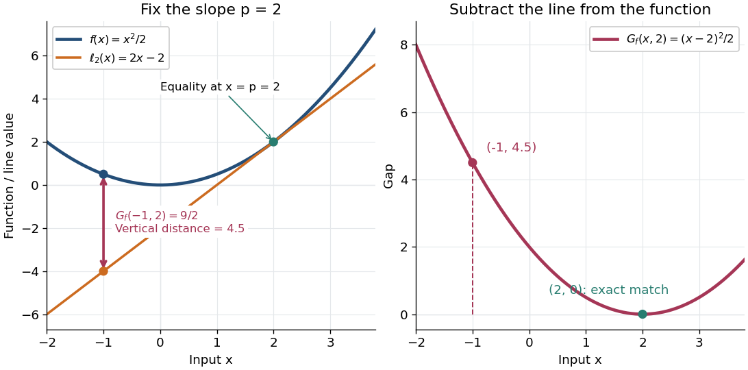
The Fenchel–Young gap is the nonnegative discrepancyfor a proper convex function and its convex conjugate. It can be $+\infty$. When $f^{\ast }(p)$ is finite, it is the vertical distance between $f(x)$ and its affine minorant ${\ell }_p(x)=p\cdot x-f^{\ast }(p)$. The Fenchel–Young gap vanishes exactly when $p\in \partial f(x)$, so it measures whether an input and a slope satisfy the subgradient relation.

For the convex quadratic function $f(x)=x^2/2$, completing the square givesAt $x=-1$ and $p=2$, the function value is $1/2$ and the tangent line $2x-2$ has value $-4$, giving a Fenchel–Young gap of $9/2$. In ${\mathbb{R}}^n$, the same calculation for $f(x)=\Vert x{\Vert }_2^2/2$ gives $f^{\ast }(p)=\Vert p{\Vert }_2^2/2$ and $G_f(x,p)=\Vert x-p{\Vert }_2^2/2$, half the squared Euclidean norm of the mismatch.

An exact optimization error certificate. Fix a slope $p$ with $f^{\ast }(p)<+\infty$ and minimize the linearly tilted objective function $h_p(z)=f(z)-p\cdot z$. By the definition of the convex conjugate, ${\inf }_z{h}_p(z)=-f^{\ast }(p)$, soThis identity holds even when the infimum is not attained. Thus a computed finite Fenchel–Young gap is exactly the error in objective value for this minimization problem. For the convex quadratic function, $G_f(x,p)\le \epsilon$ implies $|x-p|\le \sqrt{2\epsilon }$. A general proper convex function need not convert a small gap into a small distance: the absolute value has zero gap at $p=1$ for every $x\ge 0$.

The Fenchel–Young gap also connects convex analysis to optimal transport. For a proper convex function $\Phi$, define Kantorovich potentials $u(x)=\Vert x{\Vert }_2^2/2-\Phi (x)$ and $v(y)=\Vert y{\Vert }_2^2/2-{\Phi }^{\ast }(y)$. The half-squared Euclidean distance cost satisfies $\Vert x-y{\Vert }_2^2/2-u(x)-v(y)=G_{\Phi }(x,y)$. For a transport plan with finite integrated cost and integrable Kantorovich potentials, integrating this identity gives the difference between transport cost and the potentials' bound. This is the same local subgradient mismatch summed over transported pairs.

For continuous functions $f,g$ on a compact metric space satisfying $f(x)+g(y)\le d(x,y)$, set $h(x)={\min }_y(d(x,y)-g(y))$. The triangle inequality makes $h$ $1$-Lipschitz, while the constraint gives $f\le h$ and evaluation at $y=x$ gives $g\le -h$. Thus the feasible pair $(h,-h)$ has at least as large an objective against any two probability measures. This explains why metric optimal transport duality reduces to a single $1$-Lipschitz function.

Use the Lipschitz constant convention $\Vert f{\Vert }_L={\sup }_{x\ne y}|f(x)-f(y)|/d(x,y)$ in the final quantity; it is a seminorm, with constants having value zero. Also interpret the coupling space as $\mathcal{P}(X\times X)$. The printed $\mathcal{P}(X,Y)$ has an undefined $Y$. The third quantity has a duplicated printed label; it is placed in part iii here, with the fourth in part iv.

First prove weak optimal transport duality. For any feasible continuous pair $f,g$ and any coupling of probability distributions $\pi$ with marginals $P,Q$,Taking the supremum over pairs and infimum over couplings gives $m_d(P,Q)\le W(P,Q)$. These quantities are finite: $P\otimes Q$ is a coupling and the continuous cost $d$ is bounded on the compact metric space $X\times X$. The zero pair is feasible, so $0\le m_d\le W\le \mathrm{diam}X$.

The reverse inequality is established in part ii by finite approximation and a proof of the required finite linear programming duality. Parts iii and iv then show that all the dual formulations agree.

The transportation problem minimizes linear shipping cost while matching prescribed row supplies and column demands.

This is the finite discrete optimal transport problem with prescribed supply and demand marginals.