A probability measure is a nonnegative, countably additive measure with total mass one. Thus , and for pairwise disjoint events ,The complement of an event has probability . The probability of a union of overlapping events needs a correction: . Counting the overlap once is the simplest instance of the inclusion-exclusion principle.
A zero-probability event need not be impossible as a member of the sample space. Under the continuous uniform distribution on , every individual point has probability zero, while the whole interval has probability one. Countable additivity applies to countable unions, not arbitrary uncountable ones; there is no contradiction.
Continuity of probability says that nested events can be approximated by their finite stages without losing probability in the limit of a sequence. In a probability space , let . ThenThe sigma-algebra ensures that both limiting events belong to . These are continuity from below of a measure and continuity from above of a measure. The first holds even for an infinite measure; the second requires finite measure of the first set, which is automatic for a probability measure because .[ref]
For a concrete model, toss a fair coin through a sequence of independent Bernoulli trials, and let be the event of at least one head in the first tosses. Its complement is the event of initial tails. On the sample space of infinite head-or-tail sequences,Every finite waiting horizon has positive tail probability, yet the event of waiting forever has probability zero. That intersection is not empty: it contains the all-tails sequence. Thus a zero-probability event need not be impossible as an outcome, and eventual success almost surely does not supply a deterministic deadline. The waiting time for the first head has a geometric distribution with success probability . After ten tosses, the remaining tail probability is exactly ; nine tosses leave .
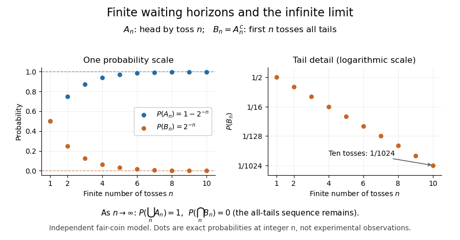
Exact fair-coin model: success by toss n increases to probability one, while the all-tails prefix probability decreases to zero
. Details. A proof outline exposes what makes countable additivity stronger than finite additivity of a set function. For increasing events, put and for . These set differences are pairwise disjoint events, their union is , and the first pieces have union . ConsequentlyFor decreasing events, their complements increase to ; applying the increasing result and the complement rule of probability gives . The finite-total-mass condition is essential for this subtraction. For comparison, the counting measure of each set of natural numbers is infinite, although their intersection is empty and has measure zero.
Conversely, on a sigma-algebra, a nonnegative normalized set function satisfying finite additivity of a set function and satisfies countable additivity. For pairwise disjoint events with , the remainders decrease to the empty set, andTaking the limit of a sequence recovers the infinite sum. This equivalence explains why continuity of probability is part of the foundations rather than a separate assumption about smooth curves.
One useful application controls infinitely many possible errors. If events satisfy , then the events decrease, and the union bound gives . Continuity of probability therefore makes : errors occur infinitely often with probability zero. This is the Borel-Cantelli first lemma, and it requires no independence. For the illustrative bounds , the probability of any error at index or later is at most , an explicit truncation guarantee.
The word continuity here concerns nested sets, not the absence of atoms in a probability distribution. For any real-valued random variable , the events decrease to . Hence its cumulative distribution function is right-continuous even when it has jumps, as for a geometric distribution. The nesting hypothesis matters: an arbitrary sequence of events need not admit either displayed interchange of limit and probability.
A probability measure is tight if compact sets carry arbitrarily nearly all its mass. Every Borel probability measure on a Polish space is tight. The stronger family condition is uniform tightness.
For càdlàg processes on a finite horizon, compact containment together with uniformly small increments over pairs of bounded stopping times whose separation tends to zero is a sufficient criterion for tightness in the Skorokhod J1 topology. The increment condition is in probability, not merely at deterministic times. If in addition the largest jump tends to zero in probability, every limiting law is supported on continuous paths.
The same compact set must work simultaneously for every measure in the family. Prokhorov's theorem relates this condition to relative compactness for the weak topology of probability measures on a Polish space.
A tight sequence of probability measures on the real line has a subsequence whose cumulative distribution functions converge at every continuity point of a cumulative distribution function. Choose a diagonal subsequence converging at every rational , write those limits as , and define . Monotonicity gives right continuity, and tightness of probability measures gives limits zero and one at the two ends of the real line. Bracketing by rational continuity approximations proves convergence at the continuity points of . The corresponding probability measure is the weak subsequential limit: approximate a bounded continuous test function by step functions on a compact interval, and use tightness to bound the tails.
A zero-probability event has probability measure zero. It need not be empty: for a continuously distributed random variable, equality with a specified value is such an event. The complementary event occurs almost surely.
For observations or orbit points , the empirical measure is . Integrating a test function gives its sample average. For orbit points , the difference between and telescopes to , so on a compact metric space with continuous , every weak limit is invariant.
If finite Borel measures and on satisfyfor every compactly supported continuous function , then . This follows from the uniqueness part of the Riesz representation theorem; alternatively, continuous functions that approximate indicators from above and below recover the measure of every interval and hence every Borel set.
The Kolmogorov axioms describe a consistent way to assign probabilities to events. Start with a sample space and an event sigma-algebra : it contains and is closed under complements and countable unions, hence also countable intersections. The probability measure is a function satisfyingThe triple is a probability space. The third axiom is countable additivity; the infinite series means the limit of a sequence of nonnegative partial sums. It applies to pairwise disjoint events, not to overlapping events and not to arbitrary uncountable unions.[ref]
The sigma-algebra specifies which questions have probabilities, while the axioms specify how those probabilities fit together. For a finite sample space one can take the entire power set; a continuous model commonly uses a Borel sigma-algebra. Nonnegativity and normalization do not require equally likely outcomes or independence: those are additional modelling choices.
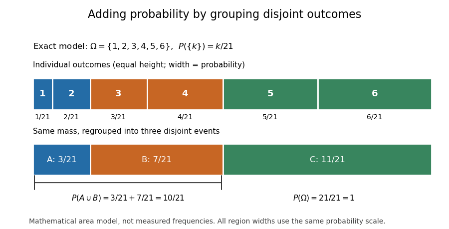
For an exact six-outcome model, take , , and assign . The total is one because . Define the probability of an event by summing the weights of its outcomes. The disjoint events , and form a partition of a set withThis is a specified mathematical model, not measured die frequencies. The figure makes probability literal area: each region has the same height and a width proportional to its assigned mass. Regrouping disjoint events preserves their total area.


Several familiar rules are consequences, not further axioms. Finite additivity of a set function follows by appending empty events to the sequence in countable additivity; follows already by writing as a disjoint union. The complement rule of probability gives and therefore . Splitting larger events into a smaller event and a set difference shows .
For overlapping events, the inclusion-exclusion principle corrects double counting:In the six-outcome model, and give , agreeing with the weight of . This decomposition is useful because a complicated event can be assembled from simpler questions with known probabilities.
On a finite sample space, a family of pairwise disjoint events has only finitely many nonempty members, so finite additivity of a set function already handles every countable disjoint union. On an infinite sample space, the countable axiom additionally controls what is left beyond every finite stage. In the fair-coin waiting model of continuity of probability, the finite-stage calculations sum to through toss . Countable additivity makes the probability of a head at some finite toss equal to ; finite-stage sums alone do not justify that passage. For the continuous uniform distribution on , each singleton instead has probability zero, while their uncountable union has probability one. Countable, rather than unrestricted, additivity accommodates both models.
Historically, Kolmogorov's 1933 book Grundbegriffe der Wahrscheinlichkeitsrechnung established the influential axiomatic framework connecting probability theory with measure theory. The three conditions above are the modern presentation on a sigma-algebra. Shafer and Vovk's historical study explains that the original presentation began with finite additivity on an algebra of sets and added continuity for decreasing events with empty intersection, which supplies the countable extension.[ref]
Let be a countable measurable partition of the sample space, with positive probabilities. For any event , the law of total probability givesThe pieces are disjoint events, so add their masses and use the definition of conditional probability. Zero-mass partition pieces can be omitted without changing the answer.
For the coin selection in probability, let mean the -head coin was selected and let mean the first toss was heads. Then . Each conditional answer describes one possible hidden situation; its weight describes how often that situation occurs under the model. This decomposition is useful whenever a simple conditional model sits behind a more complicated marginal probability distribution.
Articles by others on the same topic
There are currently no matching articles.