Let . Expanding the proposed local relation gives . Choose the derivative terms in to cancel the mixed spectral terms:Indeed,so the resulting divergence is exactly . This establishes the identity for every complex spectral parameter , with the given differentiability. The cubic dispersion relation has the reverse sign from the usual convention; that sign affects both the spectral sectors and the number of required boundary conditions.
Use the Half-range Fourier transform and the finite-time spectral boundary transformswhere for . The spatial transforms are holomorphic in , while these finite-time transforms are entire functions. For now is an unknown boundary trace. Integrating the local relation over the half-strip, using spatial decay at infinity, gives the global relationThe boundary sign follows from integrating the flux derivative: its contribution is minus the flux at zero.
Fourier inversion first gives the initial real-line integral plus a real-line integral of . To put the boundary contribution on its useful complex contour, defineOrient its full boundary with on the left. It consists of the real axis from left to right and the upper curve from right to left. The real-axis piece must not be discarded for this dispersion. The contour integration representation isTo justify the replacement, the integral of along is zero by closing above . In that region , and each boundary term is an integral of over times a polynomial in . This has no growing temporal exponential there; suppresses the upper closing arc for . The Cauchy integral theorem then applies. The figure shows the full contour and, separately, the sectors used in the nonlinear problem.
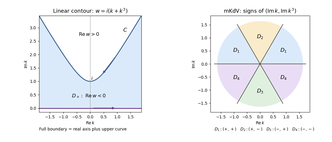
Full cubic-dispersion contour and bounded-column sectors for reverse-dispersion mKdV
. Details. 
One may replace by for any finite . Their difference is a future-time integral over ; its factor decays inside , so its integral around vanishes. All contour formulas are understood as limits of truncated contours, with standard small displacements if a boundary transform needs an Abel limit. Compatibility of the initial and boundary data controls the corner behavior. This is the two-trace half-line cubic dispersion representation.
The other roots of satisfyFor , select the unique other root with negative imaginary part. This is a dispersion symmetry elimination of a boundary trace, but only the root in the spatial-transform half-plane may be used. The root is holomorphic throughout : the upper branch point lies above its boundary. Near the real axis one other root is above and one below; a root can cross the real axis only when , so the lower-root choice persists throughout .
Evaluate the global relation at , using the same time transforms because :Consequentlywhere the completely known spectral density isThe remaining term in the solution formula has integralIts transformed argument stays in the lower half-plane, it is holomorphic inside , and does not grow there. Spatial exponential decay closes the truncated domain. Thus the formula in part (b), with replaced by , uses only the prescribed initial value and the two prescribed boundary traces. It contains no unknown or final-time solution transform. Keeping the inadmissible upper root instead would invalidate this elimination.
For asymptotic analysis it is useful to separate the spectral density from the observation time. For a fixed horizon , already has this property. If the boundary traces extend to all positive times with suitable growth, their one-sided Laplace transforms give the infinite-horizon versionFor bounded traces these integrals converge in ; boundary values are taken by an Abel limit where needed. The finite-horizon formula permits this replacement: the tail from to infinity contributes an analytic, decaying integrand with zero integral around . The resulting spectral functions are independent of .
They can be made particularly explicit on the two contour pieces. On the real axis and upper curve, respectively,The second identity follows because is real on : the remaining roots are and . Therefore rewrite the solution asThis isolates all large-time dependence in the exponential, allowing the stationary phase method or the method of steepest descent. Along , the phase is , and its stationary points satisfy . Thus the real saddles coalesce at ; any poles arising from the boundary Laplace transforms also have to be retained during contour deformation.
The source specifies smooth boundary traces, not their large-time decay or growth. Accordingly a universal numerical long-time profile cannot be inferred. The infinite-horizon formula requires the stated additional transform hypothesis; for more general data the finite-horizon density remains valid, or an appropriately shifted Laplace contour must be used. This qualification does not leave an unknown boundary trace in the representation.
Articles by others on the same topic
There are currently no matching articles.