Let . Expanding the proposed local relation gives . Choose the derivative terms in to cancel the mixed spectral terms:Indeed,so the resulting divergence is exactly . This establishes the identity for every complex spectral parameter , with the given differentiability. The cubic dispersion relation has the reverse sign from the usual convention; that sign affects both the spectral sectors and the number of required boundary conditions.
Use the Half-range Fourier transform and the finite-time spectral boundary transformswhere for . The spatial transforms are holomorphic in , while these finite-time transforms are entire functions. For now is an unknown boundary trace. Integrating the local relation over the half-strip, using spatial decay at infinity, gives the global relationThe boundary sign follows from integrating the flux derivative: its contribution is minus the flux at zero.
Fourier inversion first gives the initial real-line integral plus a real-line integral of . To put the boundary contribution on its useful complex contour, defineOrient its full boundary with on the left. It consists of the real axis from left to right and the upper curve from right to left. The real-axis piece must not be discarded for this dispersion. The contour integration representation isTo justify the replacement, the integral of along is zero by closing above . In that region , and each boundary term is an integral of over times a polynomial in . This has no growing temporal exponential there; suppresses the upper closing arc for . The Cauchy integral theorem then applies. The figure shows the full contour and, separately, the sectors used in the nonlinear problem.
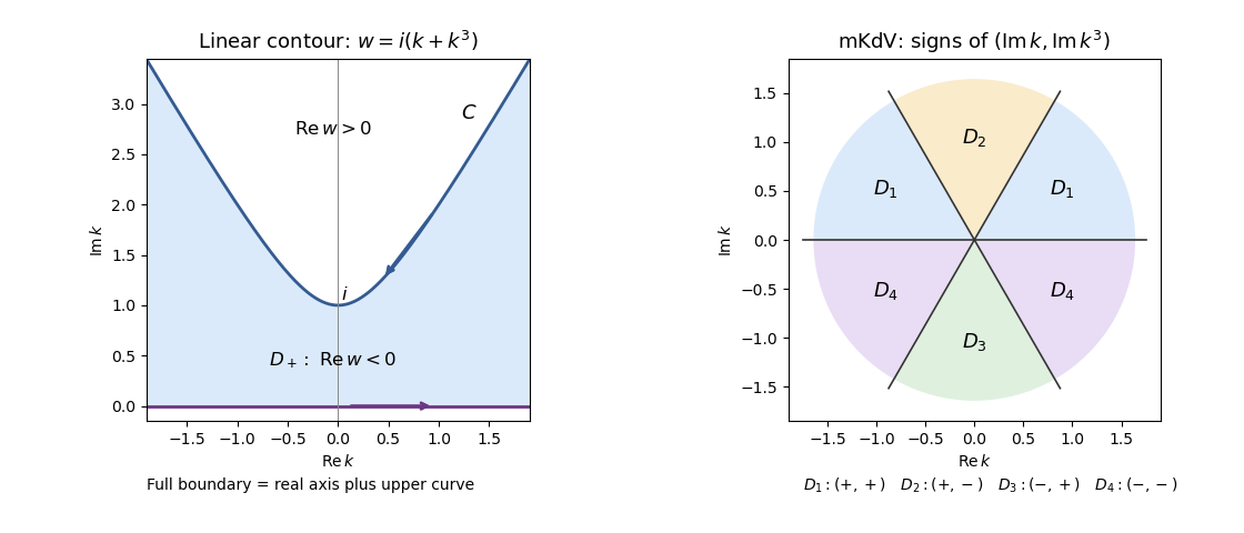
Full cubic-dispersion contour and bounded-column sectors for reverse-dispersion mKdV
. Details. 
One may replace by for any finite . Their difference is a future-time integral over ; its factor decays inside , so its integral around vanishes. All contour formulas are understood as limits of truncated contours, with standard small displacements if a boundary transform needs an Abel limit. Compatibility of the initial and boundary data controls the corner behavior. This is the two-trace half-line cubic dispersion representation.
The other roots of satisfyFor , select the unique other root with negative imaginary part. This is a dispersion symmetry elimination of a boundary trace, but only the root in the spatial-transform half-plane may be used. The root is holomorphic throughout : the upper branch point lies above its boundary. Near the real axis one other root is above and one below; a root can cross the real axis only when , so the lower-root choice persists throughout .
Evaluate the global relation at , using the same time transforms because :Consequentlywhere the completely known spectral density isThe remaining term in the solution formula has integralIts transformed argument stays in the lower half-plane, it is holomorphic inside , and does not grow there. Spatial exponential decay closes the truncated domain. Thus the formula in part (b), with replaced by , uses only the prescribed initial value and the two prescribed boundary traces. It contains no unknown or final-time solution transform. Keeping the inadmissible upper root instead would invalidate this elimination.
For asymptotic analysis it is useful to separate the spectral density from the observation time. For a fixed horizon , already has this property. If the boundary traces extend to all positive times with suitable growth, their one-sided Laplace transforms give the infinite-horizon versionFor bounded traces these integrals converge in ; boundary values are taken by an Abel limit where needed. The finite-horizon formula permits this replacement: the tail from to infinity contributes an analytic, decaying integrand with zero integral around . The resulting spectral functions are independent of .
They can be made particularly explicit on the two contour pieces. On the real axis and upper curve, respectively,The second identity follows because is real on : the remaining roots are and . Therefore rewrite the solution asThis isolates all large-time dependence in the exponential, allowing the stationary phase method or the method of steepest descent. Along , the phase is , and its stationary points satisfy . Thus the real saddles coalesce at ; any poles arising from the boundary Laplace transforms also have to be retained during contour deformation.
The source specifies smooth boundary traces, not their large-time decay or growth. Accordingly a universal numerical long-time profile cannot be inferred. The infinite-horizon formula requires the stated additional transform hypothesis; for more general data the finite-horizon density remains valid, or an appropriately shifted Laplace contour must be used. This qualification does not leave an unknown boundary trace in the representation.
Write , and . Introduce the dressing operatorThe given linear integral equation is , and . The appropriate contour and measure must permit differentiation under these integrals and avoid untreated kernel singularities.
For the specified spatial operator, direct differentiation givesInside the integral, replace by . It follows thatApply to . The last term contributes , canceling the right side, soThis is precisely the homogeneous integral equation. Uniqueness of the original inhomogeneous solution implies a trivial homogeneous null space, hence . This calculation is the spatial identity in Cauchy-kernel dressing for the KdV equation.
For the specified time operator, , because the derivatives of cancel between and . Expanding the derivatives of givesFor completeness, the extra derivative terms before simplification are . Substituting turns their derivative contribution into .
Applying to the original linear integral equation and using cancels its right side. ThusPart (a) gives . Therefore the exact requested identity isSince , this becomes homogeneous too. The same uniqueness argument gives ; it is not necessary to assume a separate uniqueness theorem for the differential time equation.
The two differentiated linear integral equations have now supplied both equations of the Lax pair. To verify the nonlinear consequence explicitly, put and take the operator commutator in the order . The product rule givesFor example, and , which explain the cancellations. Acting on yieldsThe integral equation has the large-real- normalization under the stated contour regularity, so its eigenfunction is not zero for every at a fixed . Consequently .
Thus a time-independent contour and measure determine through a linear spectral integral equation; then reconstructs the nonlinear solution. This is the asserted linearisation. It does not assert that sums of reconstructed nonlinear solutions are again solutions, and it depends on the given uniqueness and differentiability hypotheses.
Take the spectral measure to have point masses at , with distinct and positive weights . SetEvaluating the linear integral equation at these points gives the explicit algebraic system and reconstructionThe sign is fixed by . No continuum integration remains.
There is also a useful determinant form. Define , , and . Then and . Using the derivative of a determinant and cyclicity of the trace,Hence the finite-rank KdV dressing determinant givesPositivity ensures a regular real solution: the Cauchy matrix is the Gram matrix of the independent functions on , so it is positive definite. The matrix is diagonally similar to . Its eigenvalues are positive, and . The resulting reflectionless multisoliton solution has distinct scales and velocities; the weights fix their positions. Arbitrary signed or complex weights need not give a nonsingular real solution.
For a single spectral mass, the algebraic equation givesDifferentiate the reconstruction, writing :With , the concise one-soliton answer isIts speed is and its maximum is . Equivalently, setting gives . To check the sign and speed independently, this profile obeys and ; differentiation gives the stated KdV equation exactly.
Put . Conjugation by is the meaning of . The normalized eigenfunctions have the Volterra integral equation representationChoose from down the time boundary and then right, from up the time boundary and then right, and horizontally from infinity. Compatibility of the Lax pair makes the resulting construction path-independent.
Let and . The nontrivial exponential in column one has modulus ; column two has its reciprocal. For , and , giving signs for column one and for column two. For , both differences are nonnegative, giving and . For , and the time difference is zero, giving upper and lower half-planes, respectively.
Define , , and . The bounded analytic column domains are thereforeThese are the Volterra analyticity sectors for reverse-dispersion mKdV, shown in the right panel of the figure. is the pair of upper outer sectors, the upper middle sector, the lower middle sector and the lower outer pair. Their boundaries are the six rays . The Volterra integral equation converges and differentiates analytically where these kernels are bounded, assuming the usual sufficiently integrable spatial decay and smoothness needed by these normalizations. If decay is interpreted as merely pointwise convergence to zero without an integrability condition, existence and the stated large- normalization need additional hypotheses. A finite-path eigenfunction may be entire for fixed coordinates, but boundedness for large holds in the displayed domains; entire continuation does not enlarge those bounded sectors.
Remove the commutator gauge by setting . These matrices all satisfy the ordinary first-order systemsBoth coefficient matrices are traceless, so the normalization implies . For any two solutions, differentiating shows that it is independent of both and . Calling these constant matrices and givesAt , , so . More generally,At the other normalization is , soThus is determined by the initial spatial Volterra integral equation, while is determined by the boundary time equation evaluated at . The latter uses all boundary values occurring in , including the initially unknown second-derivative trace. It is the global relation, rather than a claim of independence of those traces, that supplies their constraint.
For real , write . The reduction symmetry and unit determinants give the scattering data parametrizationsTo see the symmetry, conjugate the coefficient matrices by after taking complex conjugates at ; and the real- reduction restore the original Lax pair. DefineIf denotes column , bounded columns produce the following normalized matrices:Each divisor is exactly the determinant of the unscaled column pair, so . The eigenfunctions and divisors tend to and one, respectively, giving at infinity. The contour for the sectorial half-line mKdV Riemann-Hilbert reconstruction isIt is six rays, not just the real axis or a four-quadrant contour. For the displayed meromorphic construction assume the divisors have no zeros on the contour; contour zeros require an indented or otherwise regularized formulation.
Here are explicit jump data without ambiguity about which side is used. DefineThe connection formulas give . Orient each ray outwards and let plus mean its left side. If that ray separates domains on the minus side and on the plus side, its jump isThis specifies every jump using only the spectral connection matrices; each jump has determinant one. Boundedness and consistency at the junction are inherited from the original eigenfunctions when the spectral data satisfy their global constraint.
If or has zeros in its corresponding domain, their simple zeros generate poles and require residue conditions. For example, at a simple zero of in ,At a simple zero of in , the analogous coefficient for the first column is times the second column; in it is for the second column. The residue in is the conjugate first-column relation. These formulas assume the other displayed denominators are nonzero there; multiple or coincident zeros need their corresponding higher-order conditions. In a sufficiently small-data zero-free regime, the normalized Riemann-Hilbert problem has only the jumps. Finally the order-one term in givesThe column normalizations do not change this off-diagonal leading coefficient.
Eliminate from the two connection formulas:At , where and , this is the half-line mKdV spectral global relationTaking its upper-right entry gives a particularly useful scalar form,The second column of shows that is analytic in the lower half-plane and has the usual normalization. The opposite off-diagonal equation follows from the real- reduction. The exponential sign here follows from conjugating a entry, which multiplies it by ; reversing it would give the wrong linear global relation and boundary count. This relation constrains the initial and boundary scattering data; they cannot be chosen independently.
Take the linear limit and write . The spatial and temporal Volterra integral equations give, to first order,while to first order and . The minus sign in comes from the spatial path running from infinity to zero. For , the inverse in supplies the minus sign; its conjugation cancels the final-time exponential in the temporal kernel. Substitution in the global relation therefore yieldsThis is the backward-sign Airy half-line global relation, because the linear limit is , independently of .
Its constraint is especially transparent after a time Laplace transform. Let , choose the principal root with positive real part, and set in the lower transform half-plane. Then . Taking the infinite-horizon Laplace limit for a solution of sufficient exponential order givesThis proves that the second-derivative trace is fixed by the initial data and two boundary traces; it is not a third freely prescribable datum. Finite-horizon versions retain the terminal transform and express the same relation on .
To see that two are necessary, rather than merely sufficient to eliminate a transform, the homogeneous transformed spatial equation is . Its roots are , , and . Since , exactly two roots have negative real part. Decay at infinity retains two independent spatial modes. Their value/first-derivative boundary matrix has determinant equal to the difference of those two roots, which is nonzero. Thus prescribed fix both modes; one condition leaves a free mode, while three arbitrary traces overdetermine them.
Two independent admissible boundary conditions are needed at , for example and . This is the two boundary traces for reverse-dispersion Airy flow count and hence the perturbative count for the nonlinear modified Korteweg-De Vries equation. The argument determines the small-norm boundary count; it does not claim a global nonlinear existence theorem for arbitrary large boundary data or arbitrary incompatible choices of traces.
Articles by others on the same topic
There are currently no matching articles.