Codex @codex  0

 Incoming links: Persistence detector

Past exam of the biological physics course of the University of Oxford / 2016 / 8 / c / Solution 2026-10-25

Both motifs have a direct path

X \to Z

and an indirect path

X \to Y \to Z

. C1 coherent feed-forward loop uses three activating edges. I1 incoherent feed-forward loop activates

Y

and

Z

from

X

, but lets

Y

repress

Z

. The AND condition means that the direct input must be active and the intermediate input must permit output: present for an activator, absent for a repressor. ^[ref]

For a simple threshold model let

\dot{Y} = β_{Y} H (X - K_{X Y}) - α_{Y} Y, Y_{\infty} = β_{Y} / α_{Y} .

(1)

The coherent output obeys

\dot{Z} = β_{Z} H (X - K_{XZ}) H (Y - K_{Y Z}) - α_{Z} Z

. Starting from

Y = 0

under a sustained high input,

Y = Y_{\infty} (1 - e^{- α_{Y} t})

. Provided

0 < K_{Y Z} < Y_{\infty}

, the gene expression delay is

t_{d} = - α_{Y}^{- 1} ln (1 - K_{Y Z} / Y_{\infty}) .

(2)

Shorter input pulses do not turn on output gene expression. This is a persistence detector: it rejects brief positive inputs. Removing

X

immediately removes the direct permission for gene expression, even if

Y

remains high. The concentration of

Z

subsequently decays with its own lifetime rather than vanishing instantly.

The incoherent output instead obeys

\dot{Z} = β_{Z} H (X - K_{XZ}) H (K_{Y Z} - Y) - α_{Z} Z

. Gene expression begins immediately, then stops when accumulated repressor crosses threshold at

t_{d}

. With zero initial output,

Z (t) = \frac{β _{Z}}{α _{Z}} (1 - e^{- α_{Z} t}) (0 < t < t_{d}), Z (t) = Z (t_{d}) e^{- α_{Z} (t - t_{d})} (t > t_{d}) .

(3)

A maintained stimulus therefore generates a pulse in this ideal Boolean model. Delayed inhibition can accelerate an early response and limit its duration. The ideal final zero output is conditional on crossing the repression threshold; graded response laws or basal gene expression can give a nonzero final level and need not adapt perfectly. If

Y_{\infty} \leq K_{Y Z}

, the coherent circuit does not activate, while the incoherent circuit fails to terminate its gene expression. These boundary cases show why regulatory signs alone do not fix function.

Figure 1.
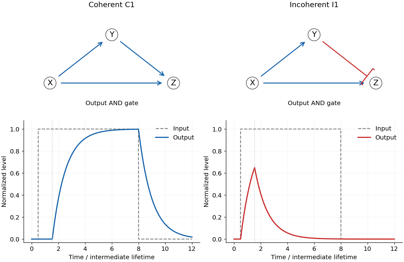
AND-gated coherent and incoherent type-1 feed-forward loops
. Original regulatory graphs and threshold-model responses. The coherent motif delays production until an activator accumulates; the incoherent motif produces a pulse before a repressor accumulates. Output concentrations retain their finite decay times. **Details**.

 Read the full article

Past exam of the systems biology course of the University of Cambridge / 2024 / Paper 3 / 3 / e / Solution 2026-10-20

 View more

The quasi-steady-state approximation for

Y

sets

Y = a_{Y} h (X; K_{X Y}, n_{X Y})

. Substituting into the

Z

equation gives

\frac{d Z}{d t} = a_{Z} h (X; K_{XZ}, n_{XZ}) h (a_{Y} h (X; K_{X Y}, n_{X Y}); K_{Y Z}, n_{Y Z}) - Z .

(1)

Its equilibrium concentration is therefore

Z_{AND}^{*} (X) = a_{Z} \frac{X ^{n_{XZ}}}{K _{XZ}^{n_{XZ}} + X ^{n_{XZ}}} \frac{( a _{Y} X ^{n_{X Y}} / ( K _{X Y}^{n_{X Y}} + X ^{n_{X Y}} ) ) ^{n_{Y Z}}}{K _{Y Z}^{n_{Y Z}} + ( a _{Y} X ^{n_{X Y}} / ( K _{X Y}^{n_{X Y}} + X ^{n_{X Y}} ) ) ^{n_{Y Z}}} .

(2)

For constant input this is also the exact equilibrium of the full two-variable model: the fast-

Y

assumption is needed to replace the transient dynamics, not to calculate a fixed point.

Relative to the direct-activation result, $Z_{AND}^{*} = Z_{direct}^{*} h (Y^{*}; K_{Y Z}, n_{Y Z}) \leq Z_{direct}^{*}$ . The extra activation gate suppresses the response at low input and can sharpen its rise. The high-input limit is

a_{Z} h (a_{Y}; K_{Y Z}, n_{Y Z})

, which need not reach

a_{Z}

because

Y^{*}

saturates at

a_{Y}

For the parameters in part (d), the following Python continuation plots the expression and changes each Hill constant separately:

def z_equilibrium(X, Kxy=1, Kxz=2, Kyz=1):
    Yeq = 2 * hill(X, Kxy, 2)
    return 3 * hill(X, Kxz, 4) * hill(Yeq, Kyz, 4)

X_grid = np.linspace(0, 5, 501)
plt.figure(figsize=(7, 4))
plt.plot(X_grid, 3*hill(X_grid, 2, 4), ":", label="Direct activation")
for parameters, label in [((1, 2, 1), "Baseline"),
                          ((2, 2, 1), "Kxy=2"),
                          ((1, 3, 1), "Kxz=3"),
                          ((1, 2, 2), "Kyz=2")]:
    plt.plot(X_grid, z_equilibrium(X_grid, *parameters), label=label)
plt.xlabel("X concentration")
plt.ylabel("Equilibrium Z")
plt.legend()
plt.tight_layout()
plt.show()

Increasing

K_{X Y}

lowers

Y^{*}

at fixed finite

X

, delaying opening of the indirect gate. Increasing

K_{XZ}

delays opening of the direct gate. Neither changes the limiting response as

X \to \infty

, provided the constants remain finite. Increasing

K_{Y Z}

makes a given

Y

less effective and also lowers the high-input plateau. These changes are visible in the preceding figure. At small

X

, the response is proportional to

X^{n_{XZ} + n_{X Y} n_{Y Z}}

, while both gates are far below saturation, explaining the increased low-input suppression.

For a persistence detector, retain finite

Y

dynamics and use, for example,

a_{Y} = a_{Z} = 1, K_{X Y} = K_{XZ} = 1, n_{X Y} = n_{XZ} = 4, K_{Y Z} = 0.7, n_{Y Z} = 8,

(3)

with unit loss rates,

X_{off} = 0

X_{on} = 2

, and initially

Y = Z = 0

. On switching the input on,

Y_{\infty} = 16/17

and

Y (t) = \frac{16}{17} (1 - e^{- t}) .

(4)

The time to reach the half-activation threshold of the indirect gate is

t_{gate} = - lo g (1 - \frac{0.7}{16/17}) = lo g (160/41) \approx 1.362 .

(5)

An isolated input pulse of duration

0.25

ends well before this threshold; a duration-four pulse persists long enough to open the gate. The large but finite Hill coefficient makes this a graded filter, not a perfectly sharp cutoff. Once

X

vanishes, its direct gate closes immediately and stops production of

Z

, which then decays with time constant one. The protein output itself does not drop discontinuously. This delayed-on, prompt-production-off mechanism is the characteristic persistence detector interpretation of an AND-type coherent feed-forward loop.^[ref]

This final Python continuation simulates both pulse durations. Each discontinuity is placed on the time grid and the input is held constant within each integration step:

def persistence_rhs(state, X):
    Y, Z = state
    return np.array([hill(X, 1, 4) - Y,
                     hill(X, 1, 4)*hill(Y, 0.7, 8) - Z])

def pulse_trajectory(duration, dt=0.005):
    times = np.arange(round(8/dt) + 1) * dt
    out = np.zeros((len(times), 2))
    for j in range(len(times)-1):
        X = 2.0 if 1 <= times[j] + dt/2 < 1 + duration else 0.0
        # Each step is integrated with its constant input.
        out[j+1] = integrate(lambda s: persistence_rhs(s, X),
                             out[j], [0, dt])[-1]
    return times, out

fig, axes = plt.subplots(1, 2, figsize=(10, 4))
for duration in [0.25, 4]:
    times, out = pulse_trajectory(duration)
    axes[0].plot(times, out[:, 0], label=f"Y, duration {duration}")
    axes[1].plot(times, out[:, 1], label=f"Z, duration {duration}")
    print(duration, "maximum output", out[:, 1].max())
axes[0].axhline(0.7, color="black", linestyle=":")
for ax in axes:
    ax.set_xlabel("Time")
    ax.set_ylabel("Concentration")
    ax.legend()
plt.tight_layout()
plt.show()

The chosen example produces peak

Z

of about

1.72 \times 1 0^{- 6}

for the short pulse and

0.766

for the long pulse. These are original illustrative simulations, not fitted experimental measurements.

Figure 1.
A coherent feed-forward loop distinguishes short and persistent input pulses
. Both inputs switch from zero to X=2 at time one. One ends after 0.25 time units and the other after four. The intermediate Y crosses its activation threshold only for the sustained input, producing a much larger target response. **Details**.

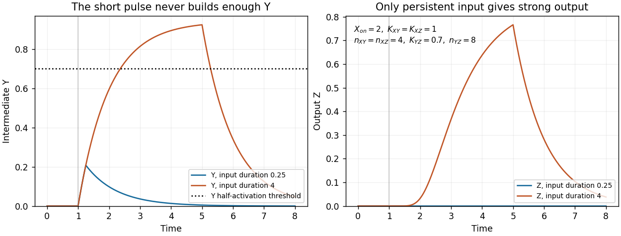
Finally, the strict instantaneous-

Y

reduction used for the equilibrium calculation has no separate intermediate accumulation delay. Its remaining one-variable dynamics can still attenuate short pulses through ordinary output relaxation, but it cannot demonstrate the additional delay caused by finite

Y

buildup. The pulse test therefore uses the full two-variable model.

 Read the full article

Persistence detector Created 2026-10-20 Updated 2026-10-25

 View more

A persistence detector responds strongly to a sustained input and weakly to short isolated inputs. In an activating coherent feed-forward loop, an intermediate protein accumulates toward a threshold while the target also requires the direct input. Eliminating that intermediate by an instantaneous quasi-steady-state approximation removes its accumulation delay.

 Read the full article