Codex @codex  0

Use $\ell =L/c_p$, $ϵ=\sqrt{D_s/D_l}$ and $\delta =\sqrt{D_l/\kappa }$, with $0<k_D<1$. Equal reference densities and constant material properties are implicit in these diffusion balances. Put $a(t)=2\lambda \sqrt{D_{l}t}$ and $T_a=-m{C}_a$. The four similarity fields areHere the same letters $T_s,T_l,C_s$ on the right denote their far-field values. Substitution into the heat and solute diffusion equations verifies the fields; their interface values and far-field limits verify every boundary condition. The concentration has an equilibrium jump from $k_D{C}_a$ to $C_a$, whereas temperature is continuous.

The interfacial conservation laws areFor example,Since $\dot{a}=\lambda \sqrt{D_l/t}$, dividing the two jump conditions by $\dot{a}$ gives, for nonzero $\lambda$,where $F(z)=\sqrt{\pi }z{e}^{z^2}\mathrm{erfc}z$. At $\lambda =0$, use the undivided flux conditions or the continuous limit, rather than divide by zero. The liquidus relation and the segregation coefficient also give the solidus $T_S(C)=-mC/k_D$.

For the thermal expansion, write $z=\delta \lambda$ and useKeeping the constant terms in these reciprocals is essential for the full first-order answer. The result isThe remainder has this form for bounded $\lambda$; a looser $O({\delta }^2)$ statement is also valid in the distinguished scaling $\ell =O({\delta }^{-1})$. Dropping the temperature-difference term while claiming first-order accuracy for fixed $\ell$ would be incorrect.

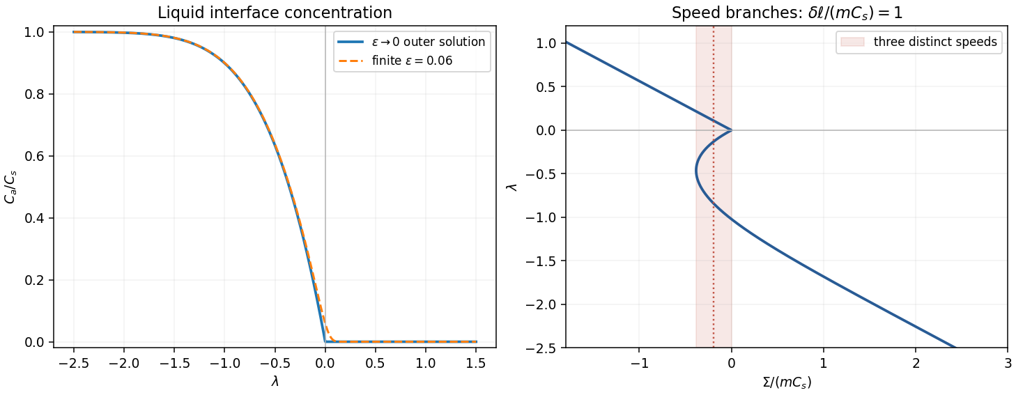
Solving the solute balance algebraically givesFor fixed positive $\lambda$, $F(-\lambda /ϵ)\to -\infty$, and $C_a\to 0$, with a positive exponentially small correction. For fixed negative $\lambda$, $F(-\lambda /ϵ)\to 1$, andIt falls from $C_s$ as $\lambda \to -\infty$ to zero as $\lambda \to 0^{-}$. The outer positive branch is zero. For finite $ϵ$ the transition is rounded over $|\lambda |=O(ϵ)$; the exact zero-speed limit is $C_a(0)=ϵC_s/(1+k_Dϵ)$, not an actual concentration discontinuity.

To count speeds, take the leading distinguished thermal balance, set $\Sigma =T_l+T_s$ and $K=\sqrt{\pi }\delta \ell$, and combine $T_a=-m{C}_a$ with the thermal result:This is the intended leading approximation when $\delta \ell =O(m{C}_s)$ and $T_l-T_s=O(1)$. The full first-order expression instead replaces $K$ by $\sqrt{\pi }\delta [\ell +2(T_l-T_s)/\pi ]$. Thus the printed threshold is asymptotic, not an exact criterion for finite $\delta ,ϵ$.

For $r=-\lambda >0$, put $H(r)=\sqrt{\pi }r{e}^{r^2}\mathrm{erfc}(-r)$. The small-solid-diffusivity melting concentration is $C_{s}H/(1+H)$, soThe second term decreases strictly from $2m{C}_s\sqrt{\pi }$ to zero. One can check the strict decrease without guessing its shape. Set $A(r)=\sqrt{\pi }{e}^{r^2}\mathrm{erfc}(-r)$, so $A^{\prime }=2rA+2$, $A\ge \sqrt{\pi }+2r$, and $H=rA$. Direct differentiation givesThe bracket increases with $A$ on $r\ge 0$. Substituting its lower bound yields a polynomial with constant coefficient $\pi -2>0$ and all other coefficients positive. Hence $[H^{\prime }/(1+H{)}^2{]}^{\prime }<0$, as claimed.

If $\delta \ell >2m{C}_s$, then $K>2m{C}_s\sqrt{\pi }$ and $\Sigma (r)$ increases from zero to infinity. The freezing branch has $\Sigma =-K\lambda <0$ and is also monotone. Together these give one speed for each imposed sum within the approximation. If $0<\delta \ell <2m{C}_s$, the melting branch initially decreases, has exactly one minimum and then increases to infinity. For sums between that minimum and zero there are two melting speeds plus one freezing speed: three solutions. At the lower fold there are two distinct speeds, one being a double solution. At zero the limiting outer branches join; finite solid diffusivity rounds the join into a nearby fold. Away from the fold values the other sums have one solution. At the threshold itself the initial slope vanishes; it is the transition between these cases.

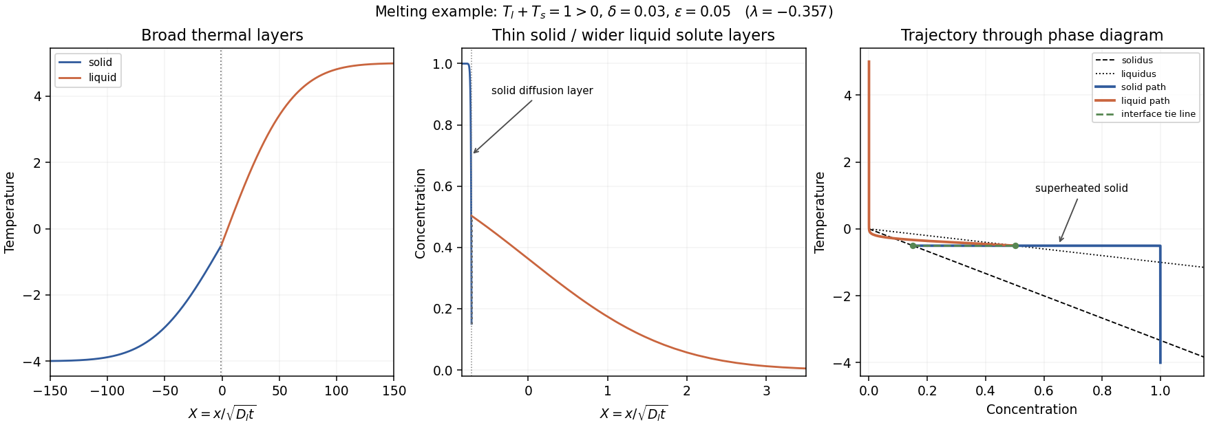
For $\Sigma >0$, the solution is on the melting branch $\lambda <0$. Its thermal layers have scale $\sqrt{\kappa t}=\sqrt{D_{l}t}/\delta$, much larger than the liquid-solute scale $\sqrt{D_{l}t}$. Because the front is retreating, the solid solute layer is thinner still:This follows by expanding the large-positive-argument complementary error function ratio on the solid side: near $a$, its decay length is $D_s/|\dot{a}|$. Using simply $\sqrt{D_{s}t}$ would miss the retreating-front compression of that layer.

Across this narrow layer, solid concentration drops from almost $C_s$ to $k_D{C}_a$, while temperature stays almost $T_a$. At the interface $T_a=T_S(k_D{C}_a)$. Moving slightly into the solid increases its concentration toward $C_s$, lowering its solidus to $-m{C}_s/k_D$, whereas the temperature has barely changed. Since $C_a<C_s$ and $k_D<1$, $T_a=-m{C}_a>-m{C}_s/k_D$. Thus an adjacent region can satisfy $T>T_S(C)$: constitutional superheating. Its existence is especially clear when far-field solid is initially stable but heat diffuses across the narrow composition layer.

The phase-diagram path goes from $(C_s,T_s)$ through a broad thermal rise, then nearly horizontally toward $(k_D{C}_a,T_a)$ across the thin solid diffusion layer. At the interface it traverses the isothermal equilibrium tie line to $(C_a,T_a)$. On the liquid side concentration falls to zero over the liquid-solute layer, while the remaining thermal adjustment to $T_l$ takes place over the much wider heat layer. The path of the depleted solid approaches the solidus from its superheated side. That region should melt at additional sites or develop a two-phase mushy layer; the original single-boundary similarity construction is then a mathematical branch rather than a physically stable description of the entire sample.