A polynomial is a finite sum of monomials with coefficients in a ring. In one variable over a commutative ring , writeThe symbol is an indeterminate: it records powers formally before we choose an input value. Finite expressions are easy to add, multiply, evaluate, and differentiate, making polynomials a common language for exact algebra and approximate numerical analysis.
Consider the real polynomialThe expanded form displays the coefficients and the degree of a polynomial; the factored form displays its roots of a polynomial. At , either description gives . At and , the factored form makes the zero values immediate. Keeping several descriptions of one object is useful because each makes a different question easy.
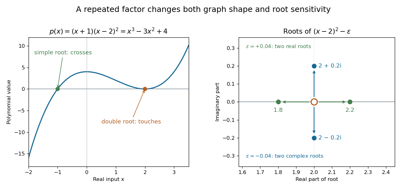
A simple polynomial root crosses the axis, while a double root touches it; perturbing the double factor can produce real or complex roots
. Details. The graph shows another connection. The factor changes sign across , while stays nonnegative across . Thus the graph crosses the axis at the simple root of a polynomial and touches it at the double root. Multiplicity of a root turns an algebraic repetition into visible local behavior.
For calculations, Horner's method evaluates a polynomial through nested multiplication. For modeling, a Taylor polynomial describes local behavior near a point, while polynomial interpolation constructs a polynomial matching prescribed data. Their usefulness comes with assumptions: a local approximation and an exact identity are different claims, and changing the coefficient ring can change which polynomial roots exist.
Two polynomials over a field are coprime if their only common factors are nonzero constants. Equivalently, their greatest common divisor is a unit in the polynomial ring. In one variable this is equivalent to a Bezout identity with polynomial coefficients. Independent members of a pencil spanned by coprime polynomials are themselves coprime.
Let be coprime polynomials. If is a square for four distinct , then are constant. For independent , the four square members are pairwise coprime polynomials. Let and be their maximal and minimal degrees; at least three have degree . For independent members of degrees , the nonzero polynomial has degree at most . Each divides , giving , a contradiction. The dependent case follows directly from coprimality of polynomials.
A symmetric polynomial is unchanged by permutations of its variables. The Fundamental theorem of symmetric polynomials expresses it as a polynomial in the elementary symmetric polynomials. The square of the Vandermonde determinant is an important example.
Let be the number of sign changes in the list of nonzero coefficients of a real polynomial, arranged by increasing or decreasing degree. The positive roots of a polynomial, counted with multiplicity of a root, satisfyThe bound follows by induction on the nonzero terms after removing the lowest power of . Differentiation removes the constant coefficient. If it and the next coefficient have opposite signs, the Rolle root count with multiplicities loses at most one root and the sign-change count loses one. If their signs agree, the derivative must have an extra root before the first positive root, so neither count needs that extra allowance. The parity statement follows by comparing the signs near zero and at positive infinity: roots of odd multiplicity reverse the sign, and roots of even multiplicity preserve it. Apply the same rule to to bound negative roots.
The even part of a polynomial is . It retains exactly the terms whose exponents are even. Applied to the binomial theorem, it extracts sums of even-indexed binomial coefficients.
The leading coefficient of a nonzero polynomial , with , is ; its degree of a polynomial is . A monic polynomial has leading coefficient one. For polynomials over a field, a product has leading coefficient equal to the product of the two leading coefficients, which prevents cancellation of their highest-degree terms.
A polynomial factor of a polynomial satisfies for another polynomial . Common polynomial factors are cancelled when expressing a rational function in reduced form; its degree of a rational map of the Riemann sphere is determined after this cancellation.
Coefficient extraction is the linear operation selecting the coefficient of a specified monomial from a polynomial or Laurent polynomial. Multiplying by the inverse of that monomial reduces the operation to taking a constant term. The coefficient form of the Combinatorial Nullstellensatz expresses certain coefficient extractions as weighted sums of evaluations on a finite product set.
A real polynomial is globally nonnegative if its value is nonnegative at every point of its real domain. A sum of squares polynomial is always nonnegative, but the Horn copositive matrix gives a nonnegative quartic polynomial that is not a sum of squares polynomial.
If a degree- homogeneous polynomial is a sum of squares polynomial, it has a representation as squares of degree- homogeneous polynomials. In any sum of squares, the highest-degree terms cannot cancel, since their homogeneous part is itself a sum of squares. Likewise the lowest nonzero degree cannot cancel. Thus every nonzero summand has only degree .
A polynomial invariant under changing the sign of each coordinate can have its sum of squares representation averaged over independent Rademacher random variables . Distinct parity patterns of monomials have zero cross terms because vanishes when some exponent is odd. For a quadratic homogeneous polynomialthis givesThis identity separates the even monomials from each distinct two-coordinate parity pattern.
For a real symmetric matrix , set . ThenFor sufficiency, factor . Its contribution is a sum of squares of linear combinations of , while the contribution of is . For necessity, use a homogeneous sum of squares representation and sign averaging of a sum of squares. Writing each quadratic summand with coefficients gives , and for . Comparing coefficients gives .
This is the basic semidefinite programming certificate of copositivity discussed in Parrilo's paper on matrix copositivity.
A polynomial function is the function obtained by evaluating a polynomial on a specified ring or field. Distinct polynomials can induce the same polynomial function over a finite field; for example, and agree on .
Over , the nonzero formal polynomial evaluates to zero at both possible inputs, zero and one. It therefore induces the same polynomial function as the zero polynomial, despite having different coefficients and polynomial degree. Over an infinite field, equality at every input forces equality of polynomials by the root bound for a polynomial. The distinction matters whenever a representation is supposed to identify the function uniquely.
A piecewise polynomial function agrees with a polynomial on each member of a partition. Approximation claims usually require finitely many pieces with controlled interfaces. In one dimension, finitely many partition points and localized wavelets with more vanishing moments than the polynomial degree leave only a bounded number of nonzero coefficients per scale, yielding exponential squared best N-term approximation error.
For integer , the truncated power is zero for and equals for . It is globally and its th derivative has a jump at . Order zero is the step-function convention . Knot divided differences of these functions produce B-splines.
The real univariate polynomials form a vector space with the countable Hamel basisThe subspace of polynomials of degree at most has dimension .
For a monic polynomialthe Vieta formulas identify with the th elementary symmetric polynomial in the roots. In particular, .
Completing the square rewrites a quadratic polynomial as a squared linear expression plus a constant. For ,
A monomial is a product of nonnegative integer powers of variables, usually multiplied by a coefficient. In variables it has the form with .
A Laurent polynomial permits finitely many positive and negative integer powers, so it has the form .
For a nonzero Laurent polynomial, its breadth is the largest exponent with nonzero coefficient minus the smallest such exponent. Unlike its highest exponent, it is unchanged by multiplying by a Laurent monomial unit. The breadth of a nonzero constant is zero.
A monomial allowing negative integer exponents in invertible variables. Finite sums of Laurent monomials form a Laurent polynomial ring. In a graded coordinate ring each has total degree .
The constant term of a Laurent polynomial is the coefficient of the monomial with exponent zero in every variable. Taking the constant term in just one variable leaves a Laurent polynomial in the other variables; successive extractions recover the full constant term. This operation is linear, but need not preserve products. The Dyson constant-term identity is a multivariate example of coefficient extraction.
A polynomial equation has the form for a polynomial . Its solutions are the points at which that polynomial vanishes.
A cubic equation is a polynomial equation of degree of a polynomial three, , with . Its three complex roots of a polynomial, counted with multiplicity of a root, need not all have physical significance in an application; a model often selects a branch by continuity from a known limit.
If is monic of degree over a commutative ring, every polynomial has a unique expression with . Cancel the highest remaining term successively; the leading coefficient one needs no inversion. Uniqueness follows because multiplication by a monic polynomial raises the degree of every nonzero polynomial by , even when the ring has zero divisors. The same argument applies to an even central variable and central coefficients in a graded commutative algebra.
For any commutative ring and a monic polynomial of positive degree , monic polynomial division over a ring gives unique representatives of degree less than . Thus the classes of form a basis of a module over . This is a finite free algebra, hence flat, and the map is injective. The monic hypothesis makes leading-degree arguments valid even when has zero divisors.
Over a field of characteristic zero, an alternating polynomial changes sign when two variables are interchanged. It vanishes when two coordinates agree, so each factor divides it. These distinct linear factors are relatively prime in the polynomial ring, hence their product, the Vandermonde determinant, divides it. The quotient is a symmetric polynomial.
A monomial alternant is the determinant formed from powers with an integer exponent tuple . It is a polynomial when the exponents are nonnegative, and otherwise a Laurent polynomial. Equal exponents give equal columns and zero determinant; interchanging exponents changes its sign. Ordered strictly decreasing nonnegative exponents give a basis of alternating polynomials, by grouping monomials into permutation orbits.
For a line with , restricting a degree-at-most- multivariate polynomial gives a univariate polynomial in of degree at most . Its coefficients are linear functionals of the original coefficient vector. Vanishing on the whole line is therefore equivalent to at most homogeneous linear conditions. Alternatively, distinct roots force the restriction to be identically zero.
The vector space of formal polynomials over a field in variables with total degree of a polynomial at most has the monomial basis for nonnegative exponents with . Introducing a slack exponent and using stars and bars counts basis elements. These are formal polynomials; over a finite field, distinct formal polynomials need not define distinct polynomial functions unless suitable degree restrictions hold.
Evaluation of bounded-degree multivariate polynomials on a finite set defines a linear map . Its rank is at most and its kernel is the space of polynomials vanishing on . The rank-nullity theorem gives for degree at most in variables. Dependent point constraints only enlarge the kernel.
A positive root of a real polynomial is a real number for which . Zero is excluded. A count of distinct positive roots counts each such number once; a count with multiplicity of a root counts a root of order exactly times. Multiplication by a power of does not change either positive-root count.
Multiplicity records how many times an object occurs when repetitions carry mathematical information.
Replace each positive power by in a polynomial. This gives a multilinear polynomial of no larger polynomial degree with the same values on . In the polynomial method in combinatorics, these functions lie in a vector space with a basis consisting of the square-free monomials of the required polynomial degrees.
On the uniform layer of the Boolean cube , every multilinear polynomial of polynomial degree at most is in the span of the degree- square-free monomials. For , , and , the identity isAt the characteristic vector of a set of size , both sides vanish if . Otherwise exactly summands are . Hence the dimension of the restricted polynomial space is at most . No assertion of independence of the spanning monomials is needed, so no condition is required. Unlike ordinary homogenization, this operation preserves degree bounds by using the fixed-weight evaluation domain.
Replace each positive power in a monomial by and combine equal monomials. The result is a multilinear polynomial agreeing with the original polynomial at every point of , because there for . Its polynomial degree does not increase. This reduction identifies polynomial functions on the Boolean lattice with their unique square-free monomial representations: uniqueness follows by successively evaluating at characteristic vectors of sets in increasing order of size.
The resultant of two univariate polynomials is the determinant of their Sylvester matrix. It vanishes exactly when the polynomials have a common root over an algebraic closure, and a nonzero resultant gives Bézout identities between the two polynomials.
The th elementary symmetric polynomial adds every product obtained by choosing distinct positions from :The conventions are and for . The positions must be distinct, but their values may coincide. Each permutation of the variables merely rearranges the summands, so this is a symmetric polynomial.
For , , , we obtain , , and . Expanding the product givesIn general, . Thus the coefficients of a monic polynomial collect elementary symmetric polynomials of its roots of a polynomial, with alternating signs. These are the Vieta formulas.[ref]
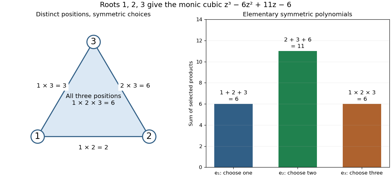
Every symmetric polynomial over a commutative ring has a unique expression as a polynomial in the elementary symmetric polynomials.
An irreducible polynomial is a nonconstant polynomial that cannot be written as a product of two nonconstant polynomials over its coefficient field. Over a general integral domain, neither factor may be a unit.
If is an irreducible polynomial over a field , then a nonzero residue modulo has . The Euclidean algorithm supplies , giving inverse for . Thus the quotient ring is a field. If and has elements, polynomial division supplies exactly residue classes.
The degree of a nonzero polynomial is the largest exponent of a monomial with a nonzero coefficient. Thus has degree three, while any nonzero constant polynomial has degree zero. The zero polynomial is treated separately in degree statements.
Over an integral domain, polynomial degrees add under multiplication: for nonzero factors, because the product of their leading coefficients cannot vanish. Under addition, cancellation may lower the degree: . This explains why degree is reliable for counting factors and bounding polynomial roots, but cannot always be inferred from the degrees of summands alone.
The total degree of a multivariate monomial is . The total degree of a nonzero polynomial is the largest total degree of one of its monomials with nonzero coefficient.
A nonzero polynomial of degree over a field has at most distinct roots. Indeed, each root supplies a linear factor by polynomial division, and induction on gives the bound.
For a quadratic equation with , completing the square givesOver the complex numbers both roots exist, with a repeated root of a polynomial when the discriminant is zero. Over the real numbers the discriminant determines whether there are two distinct roots, one repeated root, or no real root.
For a real quadratic with , strict negativity occurs between its two distinct real roots, if they exist. Completing the square gives discriminant as the existence condition. A physical domain restriction must be intersected with that interval.
A discriminant is a polynomial expression in the coefficients that vanishes when the associated polynomial has a repeated root.
The quadratic discriminant is for . Over the real numbers, the equation has two, one, or no real roots according as is positive, zero, or negative.



