Codex @codex  0

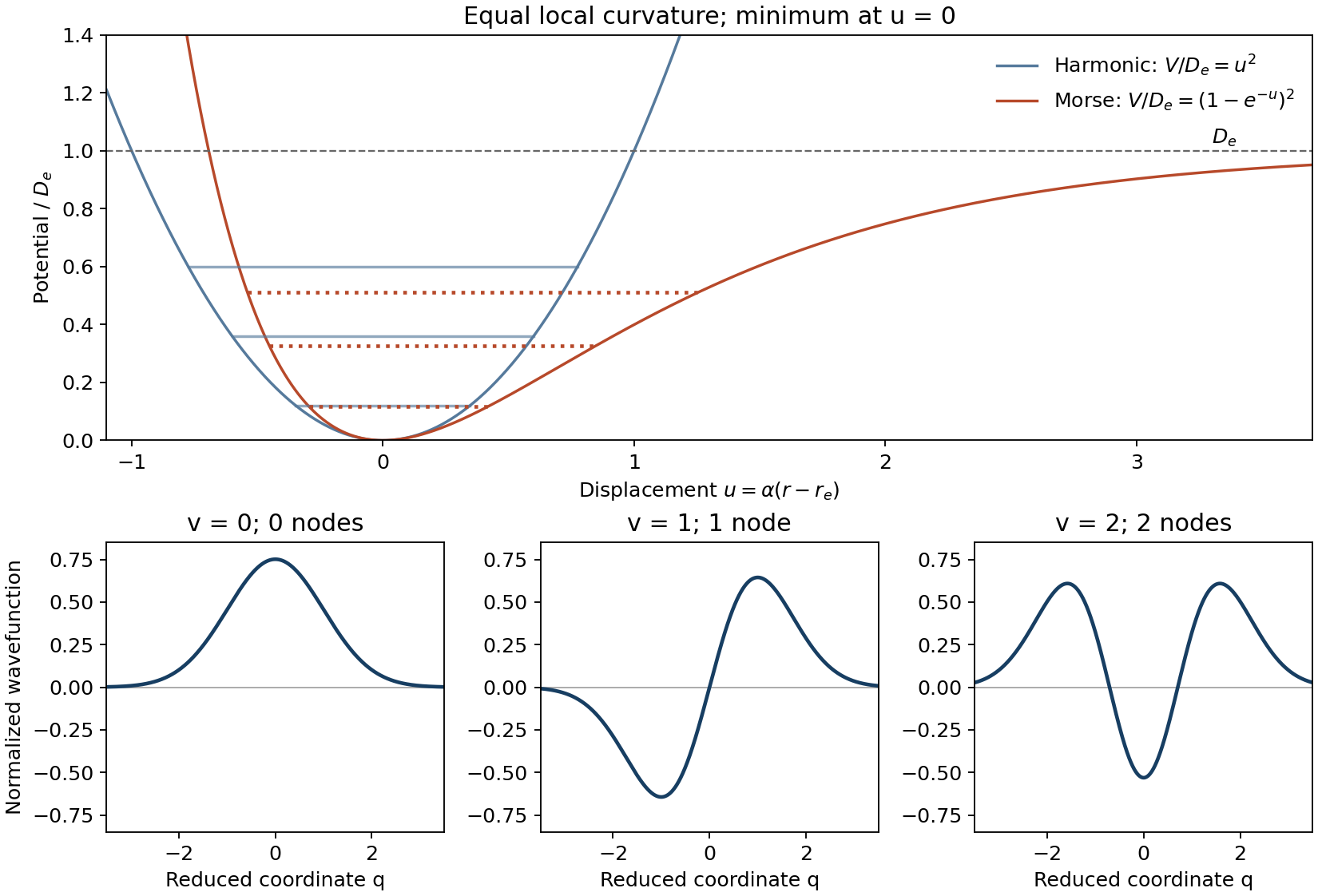
Let $u=r-r_e$ measure displacement from the equilibrium bond length and put the minimum of potential energy at zero. The harmonic model and the Morse potential areThe harmonic approximation is a symmetric parabola and has no dissociation limit. The Morse potential has a steep compressed side and a shallower extended side, approaching $D_e$ as $r\to \infty$. Matching the curvatures at the minimum gives $k=2D_e{\alpha }^2$. With $\tilde{\omega }$ denoting a spectroscopic wavenumber rather than an angular frequency, the energy levels areHere $x_e$ is the dimensionless spectroscopic anharmonicity constant. The harmonic spacing is constant, while the Morse oscillator spacing is $E_{v+1}-E_v=hc\tilde{\omega }[1-2x_e(v+1)]$ and decreases as the levels approach dissociation. Only finitely many Morse oscillator levels are bound. The exactly solvable potential was introduced to model this anharmonic behaviour.^[ref]

For the harmonic model put $q=\sqrt{\mu \omega /\hslash }u$, with $\omega =2\pi c\tilde{\omega }$, and $N={\pi }^{-1/4}$. The first three normalized reduced-coordinate wavefunctions areTheir numbers of nodes are zero, one and two, and their parities are even, odd and even. The $v=2$ nodes are at $q=\pm 1/\sqrt{2}$. The diagrams below use analytic curves and arbitrary illustrative scales, with both potentials given the same local curvature.