Codex @codex  0

Harmonic parts. Write the holomorphic function as $f=u+iv$. The Cauchy-Riemann equations say $u_x=v_y$ and $u_y=-v_x$. Equality of mixed partial derivatives therefore givesThus both the real and imaginary parts are harmonic functions and satisfy two-dimensional Laplace's equation.

Single-valued logarithm. A convenient choice isusing the principal logarithm for each term. Its branch cuts in the $z$ plane are $(-\infty ,-1]$ and $[1,\infty )$. The branch points are $-1$ and $1$: going once around the first adds $2\pi i$, while going once around the second subtracts $2\pi i$. Removing the two exterior rays makes this a consistent branch of a multivalued function and in particular leaves the whole open unit disk available.

Potential inside the cylinder. Put $z=r{e}^{i\theta }$ with $r<1$. Multiplication by $1-\overline{z}$ givesThe denominator is positive and the real part of the numerator is positive. Thus its argument lies strictly between $-\pi /2$ and $\pi /2$, andAs $r\uparrow 1$, this tends to $\pi /2$ on the upper open semicircle and $-\pi /2$ on the lower open semicircle. Scale the imaginary part to obtainIt is a harmonic function, has the required boundary values, and gives $\Phi (0)=0$. The two joining points of the boundary arcs have discontinuous boundary data, so no common continuous boundary value is demanded there. Along the real diameter, including radial approaches to either joining point, the displayed solution is zero. This is the disk potential with two semicircular boundary values.

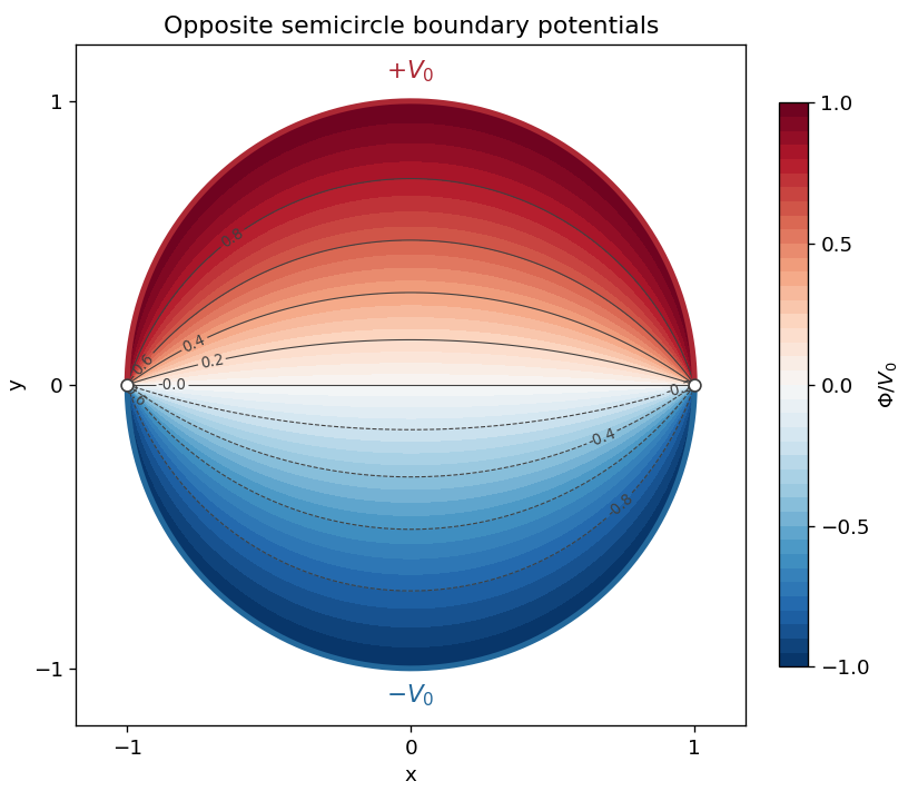
For a second check, the Taylor series of the logarithms gives $f(z)=2{\sum }_{j\ge 0}{z}^{2j+1}/(2j+1)$. Taking the imaginary part yields the Fourier serieswhose boundary limit is exactly the required alternating pair of constant semicircle values.

The coefficients in the Taylor series areFor either series, the ratio test gives absolute term ratio $|x|/(n+1)$ or $2|x|/(n+1)$, tending to zero for each fixed real or complex $x$. Both have infinite radius of convergence.

Partial fraction decomposition give $h(z)=1/(z-i)+1/(z+i)$. Let $w=z-1$. Each fraction has a geometric expansion, soEquivalently, its coefficient is $(-1{)}^j{2}^{(1-j)/2}\cos ((j+1)\pi /4)$. The first terms areThe linear and fifth-order coefficients vanish. Both geometric series converge for $|w|<\sqrt{2}$, and $h$ has genuine simple poles at $z=\pm i$, each distance $\sqrt{2}$ from the centre. Thus the Taylor series has

For the normalized second-order equation, $x_0$ is an ordinary point if both coefficient functions $p$ and $q$ are holomorphic near $x_0$. If it is singular but $(x-x_0)p(x)$ and $(x-x_0{)}^{2}q(x)$ are holomorphic there, it is a regular singular point. Thus $p$ may have at most a simple pole and $q$ at most a double pole.

The distinction tells us which local series method is justified. At an ordinary point, two independent solutions are represented by ordinary Taylor series. At a regular singular point, the Frobenius method uses $(x-x_0{)}^r{\sum }_{n\ge 0}{a}_n(x-x_0{)}^n$; the indicial equation determines the exponents, and logarithmic terms may appear in a second solution. Singularities worse than these are irregular and need not have this Frobenius form.

A simple zero of an analytic function has a local factorization $f(z)=(z-z_0)u(z)$, where $u$ is an analytic function and $u(z_0)=f^{\prime }(z_0)\ne 0$. Since $1/u$ is also an analytic function near $z_0$, its Taylor series givesThe nonzero coefficient of $(z-z_0{)}^{-1}$ proves that this is a simple pole, withMultiplying by the Taylor series $g(z)=g(z_0)+O(z-z_0)$ similarly givesThe assumption $g(z_0)\ne 0$ ensures that the pole is not canceled. In either formula the residue is precisely the coefficient of $(z-z_0{)}^{-1}$ in the Laurent series.

Put $w=z-4i$. Factor out the nonzero constant in the denominator and use the geometric series:This Taylor series converges when $|z-4i|<|3-4i|$. The simple pole at $z=3$ is the only finite obstruction to analyticity, whose distance from the expansion centre is five. Hence the radius of convergence is

Expand the exponential in inverse powers of $z$:This is a Laurent series, not a Taylor series, and converges throughout $0<|z|<\infty$. Every displayed coefficient of a negative power is nonzero, so its principal part has infinitely many terms. ThusThe residue is the coefficient of $z^{-1}$:

The Taylor series of the entire function $g$ givesThe coefficient of $(z-z_0{)}^{-1}$, and therefore the residue, isIf $g(z_0)=0$, the apparent pole is a removable singularity and the residue is zero.

For the simple-contour form of the residue theorem, let $C$ be a positively oriented, simple, closed, piecewise smooth contour. Assume $f$ is holomorphic on a neighbourhood of $C$ and its interior except at finitely many isolated singularities $z_1,\dots ,z_s$, all strictly inside $C$, with none on $C$. ThenThe more general version weights each residue by the contour's winding number, with the usual requirement that the contour be homologous to zero in the domain of analyticity containing it and the nonsingular region.

For the requested application, assume $f$ is holomorphic on a neighbourhood of the contour and its closed interior, and $z_0$ is strictly inside it. Its Taylor series showsOnly the second term contributes a residue. The residue theorem therefore proves the derivative form of the Cauchy integral formula:

For $|z|<1$, multiply the absolutely convergent Taylor series of the sine by the geometric series:The product is odd, so all even coefficients vanish. Collecting the coefficient of $z^{2m+1}$ givesFor example, the first terms are $z+5z^3/6+101z^5/120+\cdots$. The denominator vanishes at $z=\pm 1$, and the numerator is nonzero there, so these are genuine simple poles. Therefore $\boxed{R=1}$ is the radius of convergence.

If $z_0\ne 0$, factor out $z_0$ and use the geometric series:ThusThe radius of convergence is the distance to the nearest singularity, the simple pole at $z=-z_0$. The case $z_0=0$ must be treated separately: the function is $1/z$, has no Taylor series about zero and is already its own Laurent series on $0<|z|<\infty$.

The Taylor series of the logarithm givesTherefore the closed form of the larger-root Frobenius solution isThe series derivation holds initially for $0<x<1$; the closed form extends as a real solution to all $x>0$. To check it without series, put $y=\sqrt{x}v(x)$ in the original equation. All undifferentiated $v$ terms cancel and the remaining expression is $4x^{5/2}[(1+x)v^{\prime \prime }+v^{\prime }]$. Hence $[(1+x)v^{\prime }{]}^{\prime }=0$, and $v=\log (1+x)$ indeed solves it. Its logarithm is analytic near zero, so this is not a forced $\log x$ companion term at the Frobenius point.

Set $w=z-1$. Partial fraction decomposition givesExpand both terms as geometric series:The two bracketed terms are complex conjugates. Using $1\pm i=\sqrt{2}{e}^{\pm i\pi /4}$ produces the required real coefficients:The initial terms are $1-\frac{1}{2}{w}^2+\frac{1}{2}{w}^3-\frac{1}{4}{w}^4+\cdots$. The nearest singularities are the simple poles $z=\pm i$, both at distance $\sqrt{2}$ from the center. Hence the Taylor series has

A finite point $x_0$ is an ordinary point when the normal-form coefficients $p,q$ are analytic at $x_0$. Then arbitrary values $y(x_0),y^{\prime }(x_0)$ determine a convergent Taylor series, and two independent choices give two linearly independent local analytic solutions.

A singular point is a regular singular point when $(x-x_0)p(x)$ and $(x-x_0{)}^{2}q(x)$ extend analytically to $x_0$. The Frobenius method then provides at least one solutionwith a locally convergent analytic factor and an exponent fixed by the indicial equation. If its two indicial roots differ by a noninteger, there are two independent Frobenius solutions. For integer-separated roots a second solution may include a logarithm; a repeated root gives a Logarithmic Frobenius solution accompanying the single pure series. Such solutions need not be finite or ordinary Taylor series at the singular point.

Multiply the exponential power series by the two prefactors:Collecting powers yields the Laurent seriesIts first terms are $z+1+3/(2z)+7/(6z^2)+13/(24z^3)+\cdots$. Infinitely many negative-power coefficients are nonzero, so $\boxed{z=0\text{ is an essential singularity}}$. The residue is the coefficient of $z^{-1}$:The phrase "power series" here refers to a Laurent series; no ordinary Taylor series about an essential singularity exists.

The denominator vanishes at $z=\pm i\sqrt{2}$, giving two simple poles. Their distances from the center are both $|1\mp i\sqrt{2}|=\sqrt{3}$. There are no nearer singularities, so the Taylor series has radius of convergence

Seek a Frobenius solution $y=z^r{\sum }_{n\ge 0}{a}_n{z}^n$ with $a_0\ne 0$. Since $(z+z^3{)}^2=z^2+2z^4+z^6$, its lowest coefficient gives the indicial equationThus the repeated indicial root is $\boxed{r=-1}$. Equating the coefficient of $z^{n+r}$ before setting $r=-1$ givesFor $n\ge 1$ this becomes the linear recurrence relationEvery coefficient is fixed by $a_0$, since the denominator never vanishes for $n\ge 1$. In particular $a_1=0$ and then every odd coefficient is zero. Therefore there is $\boxed{\text{exactly one independent pure Frobenius series}}$, not two merely because the indicial root repeats. If "power series" means an ordinary Taylor series with nonnegative integer powers, the only such solution is zero: its coefficient equation starts with $a_0=0$ and inductively forces all coefficients to vanish.

A second independent local solution is a logarithmic solution from a repeated Frobenius exponent. Indeed, Abel's identity gives $W=C{z}^{-3}[1+O(z^2)]$. For the normalized first solution $y_1=z^{-1}[1+O(z^2)]$, reduction of order givesAfter choosing the harmless multiplicative constant in the numerator, its integrand is $1/s+O(s)$, so $y_2=y_1\log z+z^{-1}\times \text{an analytic series}$. The nonzero logarithmic coefficient proves that this second solution is not another pure Frobenius solution.

Let $K(t)=e^{tR}S{e}^{-tR}$. The product rule and differentiation of the matrix exponential givewhere brackets are the operator commutator. Evaluating at zero gives $K(0)=S$, $K^{\prime }(0)=[R,S]$ and $K^{\prime \prime }(0)=[R,[R,S]]$. The Taylor series at zero is consequentlyIn particular $[R,[R,S]]=R^{2}S-2RSR+S{R}^2$, which also follows by multiplying the two matrix exponential series through quadratic order. For fixed finite matrices the remainder has the stated Big O notation in any matrix norm.

For the first function, the complex exponential has no zeros, while the denominator has three distinct simple zeros. Thus there are $\boxed{\text{simple poles at }z=0,2i,-2i;\text{no finite zeros}}$. To examine infinity, substitute $z=1/w$:The factor $e^{1/w}$ has an essential singularity at zero, and multiplication by a nonzero finite-order factor cannot remove it. Therefore $\boxed{\infty \text{ is an isolated essential singularity}}$ of the first function.

For the second function, $\sin z$ has simple zeros at $z=n\pi$. At zero, its Taylor series givesso $\boxed{z=0\text{ is removable, with extended value }1}$. Every other $z=n\pi$ is a double pole, since the numerator is nonzero there. There are no finite zeros, including after removal at zero.

At infinity the double poles $n\pi$ accumulate. Equivalently, after $z=1/w$, the function $1/[w^2{\sin }^2(1/w)]$ has double poles at $w=1/(n\pi )$ tending to zero. Hence $\boxed{\infty \text{ is a non-isolated singularity}}$. The removable/pole/essential trichotomy for isolated singularities does not apply there; calling this an isolated essential singularity would be incorrect.

Put $w=z-1$ and $a=1-i$. Partial fraction decomposition givesBoth terms admit a geometric series at $w=0$. The local Laurent series is actually a Taylor series, since the center is regular:The nearest pole is $z=i$, a distance $|1-i|=\sqrt{2}$ from the center; the other pole is at distance $4$. Thus the requested local radius of convergence is $\boxed{R=\sqrt{2}}$.

For completeness, specifying a Laurent series without a region can also mean either of the other maximal annuli. Expanding the first fraction in inverse powers and the second in positive powers givesExpanding both fractions in inverse powers instead givesThese are different Laurent series on different annuli, rather than extensions of the local Taylor series beyond its radius of convergence.