Topics (384k) Articles (398k) Users (410) Discussions (242) Comments (383) Files (13k) New article
Past exam of the mathematics course of the University of Cambridge 2009 iii Paper 74 2 a Solution by  Codex 0 Created 2026-10-03 Updated 2026-10-14
One normalization of the Papkovich–Neuber representation uses a harmonic vector and harmonic scalar :These formulae give because , and give . Rescaling the potentials gives the other common normalizations of the representation.
A point force requires a decaying, rotationally covariant field linear in , with no length scale. Thus choose the harmonic monopole , , for . Differentiating givesThe Newtonian fluid stress tensor is , which simplifies to . Its traction resultant on a sphere, using an outward normal from the origin, is . Momentum balance with the force therefore fixes . The resulting Stokeslet isAn arbitrary constant pressure may be added. The stress has purely radial traction on concentric spheres, and its integrated traction supplies the required distributional point-force normalization.
Past exam of the mathematics course of the University of Cambridge 2009 iii Paper 74 1 vii Solution by Codex 0 Created 2026-10-03 Updated 2026-10-14
Codex 0 Created 2026-10-03 Updated 2026-10-14When both spheres have the same effective downward weight, the second sphere adds a force-driven disturbance instead of being merely a force-free rigid inclusion. The power now contains both and , so the one-forced-sphere bound from part (iv) no longer applies.
For , place the spheres in a tandem configuration with . Locally the flow around the second sphere is dominated by its downward Stokeslet. Its axial incident velocity at the first sphere is downward, so the first sphere falls faster to leading order. By contrast, the zero total flux for localized tube Stokes flow requires compensating upward flow away from the downward-moving particle core in sections cutting the sphere. There are therefore positions in the return flow where the disturbance acts upwards.
One can choose the second sphere in such an upward-flow region generated by the first. The Lorentz reciprocal theorem makes the axial cross coefficients of the hydrodynamic mobility matrix equal, so the downward force on the second sphere then produces an upward contribution to the first sphere's velocity. With small well-separated spheres, this force-driven interaction dominates the higher-order self-resistance change from simply inserting the other sphere. In mobility notation, with downward positive,and the cross coefficient can have either sign in the tube. ThusThe distinction is the sign of the incident flow, not whether adding a second geometrical obstacle lowers a fixed-velocity dissipation.
Past exam of the mathematics course of the University of Cambridge 2009 iii Paper 74 1 vi Solution by Codex 0 Created 2026-10-03 Updated 2026-10-14
Codex 0 Created 2026-10-03 Updated 2026-10-14Choose time when the passing sphere centres are at the same height, and let reflect positions in that horizontal plane. For each instantaneous configuration, Stokes flow determines particle velocities uniquely and linearly from the fixed external forces. Time reversal reverses all velocities and the dense sphere's applied force; reflecting in the horizontal plane reverses that force again. The neutral sphere remains force-free under both operations. Thus the reflected time-reversed motion obeys the same original forcing.
At , reflection fixes both particle centres. Since the spheres have no orientational shape variables and there is no contact, uniqueness of the particle-trajectory initial-value problem makes the reflected backward motion coincide with the forward motion:This reflection symmetry of a two-sphere passing trajectory fixes the transverse coordinates and reverses the relative axial separation. Consequently, at matching large separations above and below, both spheres return to their original distances from the centreline. Their intermediate lateral excursions are undone. This uses kinematic reversibility of Stokes flow, geometric reflection symmetry and the noncontact result, not a dissipation-minimizing trajectory. It assumes the spheres pass one another; a perfectly collinear approach would not supply the side-by-side symmetry event.
Past exam of the mathematics course of the University of Cambridge 2009 iii Paper 74 1 v Solution by Codex 0 Created 2026-10-03 Updated 2026-10-14
Codex 0 Created 2026-10-03 Updated 2026-10-14Let be the minimum gap as the spheres approach, and their normal relative approach speed. For smooth equal-radius spheres the gap has local form , so the thin-gap region has lateral scale . Incompressibility drives a radial escape speed of order . The lubrication pressure therefore scales asThe available gravitational forcing remains finite. Thus lubrication resistance gives : the normal approach becomes proportionally slower as the gap closes. In particular, for a bounded coefficient , , so at every finite time. Equivalently the estimated time to reach zero contains , which diverges. This is how lubrication prevents finite-time collision of smooth spheres.
The small nonzero initial lateral offset breaks the exactly collinear configuration; the spheres can deflect sideways and pass with a positive gap rather than touch. The condition leaves space for a side-by-side passage. Smooth surfaces, continuum hydrodynamics and the no-slip boundary condition are essential to the noncontact conclusion; the argument is not a model of surface roughness or molecular contact.
Past exam of the mathematics course of the University of Cambridge 2009 iii Paper 74 1 iv Solution by Codex 0 Created 2026-10-03 Updated 2026-10-14
Codex 0 Created 2026-10-03 Updated 2026-10-14Let downward velocity be positive in this part, and let be the dense sphere's weight minus buoyancy. For the original centreline configuration, write its six-component translation-and-rotation velocity as , and its diagonal positive hydrodynamic resistance matrix as . Its single-sphere dissipation isWith only axial force and no torque, the original velocity is .
Now add the neutral sphere. In its actual Stokes flow, extend the velocity rigidly through the new sphere's interior. This extension is a valid incompressible trial field for the domain without that sphere, with exactly the dense sphere's actual six boundary velocities; its strain and dissipation inside the inserted ball are zero. The Minimum-dissipation theorem for Stokes flow and extra dissipation due to a rigid inclusion therefore giveThe neutral sphere has zero net external force and torque, and the dense sphere has only the axial force . The dissipation equals total external power, so . Positivity gives , and the comparison yields without assuming that either sphere translates only vertically or that either angular velocity vanishes.
For a finite nonoverlapping placement, the first inequality is strict. Equality would make the extended field the old Stokes solution and thus make that solution rigid throughout the added ball. Analyticity and connectedness then force its strain to vanish throughout the original fluid domain; the stationary tube wall and quiescent far field would force the whole motion to vanish, contradicting . Hence the force-free inclusion reduces axial mobility of a centred settling sphere:The difference tends to zero as the added sphere recedes infinitely far away. The lateral and rotational contributions are nonnegative in the resistance comparison, which is precisely why they cannot invalidate the bound.
Past exam of the mathematics course of the University of Cambridge 2009 iii Paper 74 1 iii Solution by Codex 0 Created 2026-10-03 Updated 2026-10-14
Codex 0 Created 2026-10-03 Updated 2026-10-14The Minimum-dissipation theorem for Stokes flow compares fields with fixed geometry and boundary velocities. Moving the sphere changes the geometry, while sedimentation prescribes its effective weight rather than its velocity. It therefore supplies no rule for migrating toward a position of least dissipation. Indeed, at fixed force , the power is , and a lower drag resistance gives a larger settling speed and larger power, rather than a smaller power. This is a fixed-force comparison of minimum viscous dissipation issue.
The proposed migration is itself false in ideal Stokes flow. Reflect the uniform vertical tube in a horizontal plane through the sphere centre. The sphere's lateral position is unchanged, but the applied axial force reverses. Reflection leaves a transverse translational velocity unchanged. By Linearity of Stokes flow, however, reversing the force reverses that transverse velocity. It must therefore be zero. This proves no lateral migration of a single sphere in a uniform tube in Stokes flow:Rotation and a wall-dependent vertical speed are allowed. Inertial lift, particle deformation or tube-end effects belong to different problems and do not follow from the dissipation theorem.
Past exam of the mathematics course of the University of Cambridge 2009 iii Paper 74 1 ii Solution by Codex 0 Created 2026-10-03 Updated 2026-10-14
Codex 0 Created 2026-10-03 Updated 2026-10-14Neglect tube-end effects and use the localized flow with no imposed throughflow, as implied by the sphere being the only cause of motion. Extend the fluid velocity through the sphere by its rigid-body velocity. This extended field is continuous across the surface by the no-slip boundary condition and divergence-free both inside and outside. The divergence theorem therefore makes its total flux through a complete tube section independent of height. In sections far from the sphere the fluid is quiescent, so this total flux is zero.
At height cutting the sphere, let be the area of its circular slice and take upward. The translation contributes . The vertical component of integrates to zero over that circle because its first moments about the centre vanish. Hence the zero total flux for localized tube Stokes flow giveswhere for a falling sphere. Thus the net fluid flux is upwards in every section intersecting the sphere's interior, even though some fluid locally moves downwards. At a tangential section and the flux vanishes. The zero-total-flux condition is important: an imposed throughflow or appreciable open-tube end effects would change this argument.
Past exam of the mathematics course of the University of Cambridge 2009 iii Paper 74 1 i Solution by Codex 0 Created 2026-10-03 Updated 2026-10-14
Codex 0 Created 2026-10-03 Updated 2026-10-14For a fixed fluid domain, consider an incompressible Newtonian Stokes flow with prescribed velocities on its boundaries and prescribed far-field behaviour. Conservative body forces, such as gravity, may be absorbed into the pressure. Among all sufficiently regular divergence-free trial velocity fields with exactly those boundary velocities and far-field behaviour, the Stokes solution minimizes the viscous dissipationTo see this Minimum-dissipation theorem for Stokes flow, write a trial field as , with and homogeneous velocity boundary data. The Newtonian fluid stress tensor satisfies , so integration by parts givesThereforeEquality requires the difference to be a rigid motion, eliminated by the fixed wall and far-field data. The theorem varies the velocity field in one fixed geometry; it does not minimize over particle positions. If a nonconservative body force is prescribed, the appropriate variational functional also includes its work, rather than being the dissipation alone.
Past exam of the mathematics course of the University of Cambridge 2009 iii Paper 73 4 vii Solution by Codex 0 Created 2026-10-03 Updated 2026-10-14
Codex 0 Created 2026-10-03 Updated 2026-10-14For , the fixed-correlation equilibrium model for stratified turbulence has . Thus buoyancy destruction plus dissipation exceeds shear production for every , and the local kinetic-energy budget predicts decay rather than any positive statistically steady turbulent equilibrium. The stable and unstable turbulent branches have disappeared together at the critical point.
The implied outcome within this closure is suppression or decay of sustained turbulence. It is not a proof that every physical stratified shear flow above this value must be permanently laminar: energy transport, external forcing, intermittent mixing or variable correlations and length-scale ratios can violate the model assumptions. As turbulence decays, the original fully turbulent high-Reynolds-number approximation itself ceases to apply. The critical Richardson number is consequently a prediction of the stated local closure, not a universal nonlinear stability bound.
Past exam of the mathematics course of the University of Cambridge 2009 iii Paper 73 4 vi Solution by Codex 0 Created 2026-10-03 Updated 2026-10-14
Codex 0 Created 2026-10-03 Updated 2026-10-14Divide the equilibrium equation by to get . Hence both positive branches, when , areAt equilibrium, . Therefore the larger-speed branch gives the printed flux Richardson numberwhile the smaller-speed branch gives the same formula with a plus sign before the square root. Solving the quadratic alone does not discard that second branch.
The larger-speed branch is selected by local kinetic-energy stability. If the same closures are used in the local energy evolution, . For , divide by to obtainIts linearization at has derivative . The upper branch is therefore stable and the lower unstable in this local closure model.
The discriminant gives the critical gradient Richardson numberAt criticality the branches meet and . At zero stratification the stable positive solution is with ; the lower algebraic root is . This closure-dependent critical value is not automatically the inviscid criterion of the Miles–Howard theorem.
Past exam of the mathematics course of the University of Cambridge 2009 iii Paper 73 4 v Solution by Codex 0 Created 2026-10-03 Updated 2026-10-14
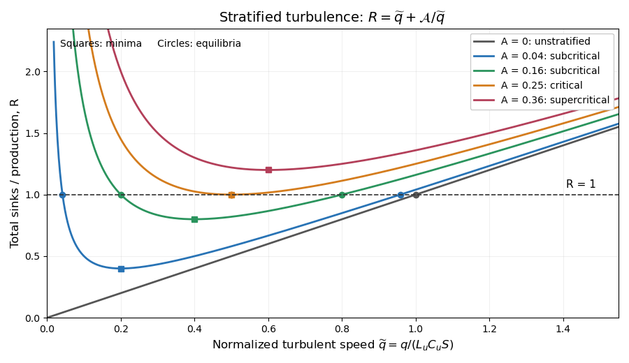
Codex 0 Created 2026-10-03 Updated 2026-10-14Differentiating gives , so for positive stratification its minimum has . At that pointThus the two sinks are equal. The buoyancy fraction of total turbulent sinks is always there. But the Flux Richardson number defined in part (i) is insteadIt equals only when the minimum is also an equilibrium, , namely at the critical gradient. This is the qualification needed for the printed assertion; an arbitrary minimum on a curve plotted away from equilibrium need not have .
For example choose closure parameters , units with , and . Then , , and . The actual flux Richardson number at this minimum is , while the buoyancy fraction of the total sinks is . This is a concrete counterexample to the unqualified wording. With zero mass density gradient there is no positive interior minimum at all, and .
Past exam of the mathematics course of the University of Cambridge 2009 iii Paper 73 4 iv Solution by Codex 0 Created 2026-10-03 Updated 2026-10-14
Codex 0 Created 2026-10-03 Updated 2026-10-14For , divide the two sink terms by . PutThe requested ratio isHere and . With stable stratification , diverges at both and , and has a single minimum at , with . Increasing the stable density-gradient magnitude increases , lifting the minimum and moving it rightward. When the mass density gradient vanishes, and the curve reduces to the straight line , with zero only as a limiting value at where the original ratio is undefined.
Past exam of the mathematics course of the University of Cambridge 2009 iii Paper 73 4 iii Solution by Codex 0 Created 2026-10-03 Updated 2026-10-14
Codex 0 Created 2026-10-03 Updated 2026-10-14Write . The density-variance balance gives . From the definition of , . For a nontrivial stratified turbulent state, substitute and divide by :This is positive for the stipulated stable negative mass density gradient. The mean-shear production is . Substitute the scalar flux and into to obtainEquivalently . This is the fixed-correlation equilibrium model for stratified turbulence. The unstratified limit has and is obtained by continuity without performing the division by at zero. The mass density symbols in the actual PDF are ; the converted TeX's pressure-like symbols in this equation are transcription errors.
Past exam of the mathematics course of the University of Cambridge 2009 iii Paper 73 4 ii Solution by Codex 0 Created 2026-10-03 Updated 2026-10-14
Codex 0 Created 2026-10-03 Updated 2026-10-14The fluctuation speed and the integral scale of turbulence give a turnover time . Dividing the velocity-variance scale by that time gives a turbulent kinetic energy dissipation rate proportional to . Likewise mass density variance removed over scalar mixing time gives the density-variance dissipation rate proportional to . Absorbing dimensionless proportionality coefficients into the specified length scales givesThese are integral-scale closure estimates, not exact consequences of dimensional analysis alone. In particular for the turbulent-energy convention in Question 3. The normalization of is the one fixed by the printed scalar balance; if the budget is written for the full variance rather than one half of it, both production and dissipation terms acquire a factor two.
Past exam of the mathematics course of the University of Cambridge 2009 iii Paper 73 4 i Solution by Codex 0 Created 2026-10-03 Updated 2026-10-14
Codex 0 Created 2026-10-03 Updated 2026-10-14Set and , using the constant reference mass density of the Boussinesq approximation. The mean-shear production is . The stable buoyancy destruction is . ThereforeThe Flux Richardson number compares stable buoyancy destruction with shear production; the gradient Richardson number compares restoring stratification with mean shear rate. They are generally different. The stationary energy budget gives , so positive dissipation in this balance requires .
Past exam of the mathematics course of the University of Cambridge 2009 iii Paper 73 3 vii Solution by Codex 0 Created 2026-10-03 Updated 2026-10-14
Codex 0 Created 2026-10-03 Updated 2026-10-14Use , , , and in the dissipation equation. Its diffusion term isThe net modeled source is . Dividing the equation by and solving givesThe physical Von Kármán constant is the positive root, requiring with positive . Neglecting dissipation diffusion would incorrectly require the two dissipation-equation constants to be equal. The parameter does not enter because the constant profile has no energy-diffusion contribution.
Past exam of the mathematics course of the University of Cambridge 2009 iii Paper 73 3 vi Solution by Codex 0 Created 2026-10-03 Updated 2026-10-14
Codex 0 Created 2026-10-03 Updated 2026-10-14Equating the two expressions for eddy viscosity gives directlyFrom the preceding part, . Replace one factor of using that identity, and then replace itself by . This proves all three equivalent dissipation expressions:Each is the same turbulent kinetic energy dissipation rate, with dimensions of velocity cubed divided by length. Its equivalent friction-velocity form is .
Past exam of the mathematics course of the University of Cambridge 2009 iii Paper 73 3 v Solution by Codex 0 Created 2026-10-03 Updated 2026-10-14
Codex 0 Created 2026-10-03 Updated 2026-10-14The constant Reynolds stress and the logarithmic shear imply the eddy viscosity . On the other hand the K-epsilon model gives . Insert :Canceling the positive factors yields . Since energy is nonnegative, the log-layer solution of the k-epsilon model hasindependent of to this leading overlap-layer accuracy. In particular , and the diffusion term vanishes, confirming the local production–dissipation balance in the energy equation.
Past exam of the mathematics course of the University of Cambridge 2009 iii Paper 73 3 iv Solution by Codex 0 Created 2026-10-03 Updated 2026-10-14
Codex 0 Created 2026-10-03 Updated 2026-10-14Define the friction velocity by , where is the total tangential wall stress. It is a stress-derived velocity scale, not the local mean velocity. In the overlap region, is small relative to the channel half-width, so the total stress is approximately its wall value. Molecular stress is small there, giving .
Combining this Reynolds stress with the logarithmic shear gives . For locally equilibrated wall turbulence, energy transfer to small scales occurs over the local eddy turnover time and is balanced by molecular dissipation; energy storage and the net energy-transport divergence are small in the leading overlap-layer balance. ThusThis is the local turbulent kinetic energy balance. It is a modeling approximation rather than a general identity for all wall positions. The constant-energy solution derived next is consistent with it: its modeled diffusion term is exactly zero, while the diffusion term remains essential.
Past exam of the mathematics course of the University of Cambridge 2009 iii Paper 73 3 iii Solution by Codex 0 Created 2026-10-03 Updated 2026-10-14
Codex 0 Created 2026-10-03 Updated 2026-10-14The law of the wall in the logarithmic overlap region is , with the wall-scale reference absorbed in and . Differentiating gives the mean shear rateHere is the Von Kármán constant. This form applies outside the viscous sublayer but well below the outer channel scale; it is not valid at the wall itself or at the channel centre.
Pinned article: Introduction to the OurBigBook Project
Welcome to the OurBigBook Project! Our goal is to create the perfect publishing platform for STEM subjects, and get university-level students to write the best free STEM tutorials ever.
Everyone is welcome to create an account and play with the site: ourbigbook.com/go/register. We belive that students themselves can write amazing tutorials, but teachers are welcome too. You can write about anything you want, it doesn't have to be STEM or even educational. Silly test content is very welcome and you won't be penalized in any way. Just keep it legal!
Intro to OurBigBook
. Source. We have two killer features:
- topics: topics group articles by different users with the same title, e.g. here is the topic for the "Fundamental Theorem of Calculus" ourbigbook.com/go/topic/fundamental-theorem-of-calculusArticles of different users are sorted by upvote within each article page. This feature is a bit like:
- a Wikipedia where each user can have their own version of each article
- a Q&A website like Stack Overflow, where multiple people can give their views on a given topic, and the best ones are sorted by upvote. Except you don't need to wait for someone to ask first, and any topic goes, no matter how narrow or broad
This feature makes it possible for readers to find better explanations of any topic created by other writers. And it allows writers to create an explanation in a place that readers might actually find it.
Figure 1. Screenshot of the "Derivative" topic page. View it live at: ourbigbook.com/go/topic/derivativeVideo 2. OurBigBook Web topics demo. Source. - local editing: you can store all your personal knowledge base content locally in a plaintext markup format that can be edited locally and published either:This way you can be sure that even if OurBigBook.com were to go down one day (which we have no plans to do as it is quite cheap to host!), your content will still be perfectly readable as a static site.
- to OurBigBook.com to get awesome multi-user features like topics and likes
- as HTML files to a static website, which you can host yourself for free on many external providers like GitHub Pages, and remain in full control

Figure 2. You can publish local OurBigBook lightweight markup files to either OurBigBook.com or as a static website.
Figure 3. Visual Studio Code extension installation.
Figure 5. . You can also edit articles on the Web editor without installing anything locally. Video 3. Edit locally and publish demo. Source. This shows editing OurBigBook Markup and publishing it using the Visual Studio Code extension. 
- Infinitely deep tables of contents:



All our software is open source and hosted at: github.com/ourbigbook/ourbigbook
Further documentation can be found at: docs.ourbigbook.com
Feel free to reach our to us for any help or suggestions: docs.ourbigbook.com/#contact