Topics (384k) Articles (398k) Users (410) Discussions (242) Comments (383) Files (13k) New article
Past exam of the mathematics course of the University of Cambridge 2009 iii Paper 63 4 a Solution by  Codex 0 Created 2026-10-03 Updated 2026-10-14
Since the donor fills its Roche lobe, use and substitute its equilibrium mass-radius relation into the lobe approximation:Kepler's third law then givesso the Roche-lobe period-mass relation for a linear donor radius law isThe total binary mass cancels, rather than being assumed equal to the white-dwarf mass.
The orbital radii about the center of mass are and . Summing the two orbital angular momenta givesWith transferred matter retained by the accretor, total mass is fixed. Logarithmic differentiation givesFor , the separation response is . Since at fixed total mass,The second relation uses the supplied equilibrium donor sequence. As the donor loses mass, . If , its Roche lobe shrinks fractionally faster than this donor radius, so the excess filling increases and drives more transfer: it is positive feedback. If , infinitesimal loss instead reduces overfill on that assumed sequence, so some continuing driver is needed to retain contact.
There are two limits to the literal dynamical interpretation. The given initial range is , so is an extrapolated instability test, not a state inside that range. Also, a true dynamical stability of binary mass transfer test needs the donor's adiabatic stellar radius response exponent , rather than its thermal-equilibrium exponent. In general,Thus is the result for the assumed response. A fully convective idealized donor has , giving a dynamical threshold , already below . The equilibrium radius law alone should not be used to assert a universal dynamical threshold.
One continuing driver is magnetic braking of a binary star. A magnetized wind carries away the donor's spin angular momentum; tides that maintain near-synchronous rotation replenish that spin from the orbit, removing orbital angular momentum. With an external , the lobe response becomesEquating this to the donor response proves the binary mass-transfer contact equation in this model:A negative torque therefore drives mass loss while maintaining contact for , subject to the chosen donor response and braking assumptions.
Past exam of the mathematics course of the University of Cambridge 2009 iii Paper 63 3 b Solution by Codex 0 Created 2026-10-03 Updated 2026-10-14
Codex 0 Created 2026-10-03 Updated 2026-10-14Use for the neon-22 mass fraction, temporarily keeping it distinct from the earlier metallicity. Let be the baryon density, ignoring small nuclear mass defects. Equal masses of carbon and oxygen giveCarbon-12 and oxygen-16 each have equal proton and neutron numbers, while neon-22 has ten protons and twelve neutrons. The total proton and neutron numbers per baryon are consequentlyHenceThe equal carbon/oxygen mass split cancels from this result: any mixture of these two symmetric nuclei has the same electron fraction. Taking the paper's metallicity symbol to mean gives its requested expression.
The literal pre-helium-burning nitrogen interpretation, however, needs a correction. Each initial nitrogen-14 nucleus receives two alpha particles, including eight additional baryons, before becoming neon-22; the intervening beta-plus decay also emits a neutrino. Thus, if the entire original metallicity is nitrogen-14 with mass fraction , conservation of the number of seed nuclei givesThis is neon-22 neutron excess from nitrogen-14. The two expressions are compatible only when their arguments are distinguished: the displayed law uses the final neon mass fraction, not literally the earlier nitrogen mass fraction. Treating those fractions as equal is an extra simplifying approximation, not a consequence of the stated capture chain.
A radioactively powered Type Ia supernova light curve rises to a broad maximum over roughly weeks as energy deposited in expanding ejecta diffuses out, then declines over the following weeks and months. Its power comes predominantly from the nickel-56 decay chain, first nickel to cobalt and then cobalt to iron. Gamma rays and charged decay products deposit heat, which is reprocessed into optical and infrared radiation. At later times, declining cobalt decay power and increasing gamma-ray escape shape the tail. It is not sustained nuclear fusion in the expanding ejecta. The amount of radioactive nickel, photon diffusion time and deposition efficiency all matter, so an uncorrected fixed luminosity is only an idealization.
For the requested two-isotope yield calculation, assume the same total processed iron-group mass, namely as inferred from the zero-neon reference. Treat the final freeze-out ashes as nickel-56 and iron-54, neglecting residual light particles and additional weak neutronization. If is the nickel mass fraction, conservation of electron fraction givesSince , this reduces to the metallicity dependence of nickel-56 yieldUnder the paper's intended identification ,If instead denotes the earlier nitrogen mass fraction, retaining the actual capture stoichiometry gives and . The same temperature and density do not alone fix a total burned mass; equality of that mass is also implicit in the comparison. The two-isotope assumption is a bulk-ash approximation, not a complete equilibrium network with all free particles identically absent.
For otherwise comparable explosions, approximate the peak luminosity by a quantity proportional to the radioactive nickel mass. Let be the true distance to an extremely low-neon event, and use the solar calibration . Its measured flux is , but the inferred standard-candle distance isThe source is intrinsically brighter than the calibration, so the distance is underestimated by about , conventionally described here as about . Equivalently, , consistent with the supplied rounded factor . Using the literal nitrogen metallicity instead gives about a underestimate. These are conditional composition effects in this simplified model; real Type Ia distance estimation also standardizes light-curve shape and color.
Past exam of the mathematics course of the University of Cambridge 2009 iii Paper 63 3 a Solution by Codex 0 Created 2026-10-03 Updated 2026-10-14
Codex 0 Created 2026-10-03 Updated 2026-10-14Write and for the number densities of nickel-56 and iron-54. Both nuclei contain 28 neutrons, while their proton numbers differ by two. Dividing the positive-exponential nuclear statistical equilibrium formulas printed in the PDF therefore gives the nickel–iron nuclear equilibrium ratioThe neutron-density factors cancel. contains the isotope-dependent statistical and translational mass factors suppressed in the supplied proportionality; it is constant in this simplified calculation. The TeX conversion incorrectly reverses the exponential sign, so the PDF sign is essential here.
In the specified restricted composition, equality of total proton and neutron numbers meansConsequentlyDifferentiation, with the suppressed prefactors held constant, givesUsing the paper's supplied signed energy difference producesWith that negative value, tends to zero at both temperature endpoints, increases below this temperature and decreases above it. At the stationary point , so it is indeed a maximum for the printed toy data.
There is a genuine physical-data qualification: the stated negative energy difference is inconsistent with interpreting as the conventional positive total nuclear binding energy of these actual isotopes. Using atomic masses, whose electron masses cancel in this reaction,The masses used are , and , from NIST hydrogen masses, NIST iron masses and NIST nickel masses. Small electronic binding corrections do not change the sign. With a positive , the simplified above is strictly decreasing for and has no finite maximum. Thus the numerical maximum follows from the supplied negative parameter, not from consistent physical binding energies; changing the TeX sign to recover a maximum would not repair the PDF's data.
Nuclear statistical equilibrium is appropriate when the relevant forward and inverse strong or electromagnetic reactions are fast compared with changes of temperature, density and composition. It is useful in sufficiently hot late silicon-burning material and in the hottest explosive burning regions of massive stars. Some burning zones reach only quasi-equilibrium, and cooling or expansion eventually freezes the abundances out; an equilibrium expression cannot by itself predict the full ashes when these timescale conditions fail. Temperature, density, conserved baryon number and the electron fraction in stellar matter must all be specified. Negligible free-particle contributions in bulk bookkeeping are not the same as exactly zero free densities in the equilibrium formula.
Strong and electromagnetic reactions preserve total charge and baryon number, so they conserve the proton-to-neutron ratio. Weak reactions need not: electron capture and beta-plus decay convert protons into neutrons and lower it. Such conversions occur in hydrogen-burning networks and in the nitrogen-to-neon chain during helium burning. At high density in advanced stellar cores and core collapse, electron capture becomes particularly important; neutrino emission also affects energy and lepton loss. Beta-minus decay changes the ratio in the opposite direction and can compete during later relaxation. Nuclear equilibrium for strong reactions does not automatically imply weak equilibrium or a fixed proton-to-neutron ratio throughout all stellar evolution.
Past exam of the mathematics course of the University of Cambridge 2009 iii Paper 62 3 b Solution by Codex 0 Created 2026-10-03 Updated 2026-10-14
Codex 0 Created 2026-10-03 Updated 2026-10-14To distinguish the moment quantity from the gravitational constant, write it as . Newton's equations give and . Differentiating provesAverage from to , divide by , and apply the supplied long-time boundary condition. The result isThe PDF's intermediate formula omits this minus sign. It cannot follow from the preceding derivative identity: an attractive inverse-square circular orbit already has and , contradicting the printed positive-sign version. The later homogeneous-potential relation is consistent with the corrected sign.
Interpret as the total pair potential energy, with each pair counted once, for example . The printed pair sum leaves one particle index unspecified; an ordered-pair convention with the corresponding factor absorbed into has the same degree of homogeneity. Under a common dilation of all positions,Differentiating with respect to at one is the Euler theorem for homogeneous functions. Since , it givesSubstitution into the correctly signed averaged identity proves the virial theorem for a homogeneous pair potential:For , the conserved total energy can be evaluated using these averages:Use the kinetic temperature convention , where for three-dimensional thermalized particles, or the same positive coefficient as a kinetic-temperature definition. At fixed particle number and interaction parameters,Thus the equilibrium heat capacity is negative precisely whensubject to existence of the bounded equilibrium sequence assumed by the virial theorem. At the virial energy is zero and this derivative vanishes. At the written power-law potential is constant, its force vanishes, and the bounded-motion virial condition excludes nonzero kinetic energy; division by is not permissible. The Newtonian case recovers .
Past exam of the mathematics course of the University of Cambridge 2009 iii Paper 62 3 a Solution by Codex 0 Created 2026-10-03 Updated 2026-10-14
Codex 0 Created 2026-10-03 Updated 2026-10-14For an isolated collisionless stellar system, define the scalar second mass moment and total kinetic energy byTake moments of the Collisionless Boltzmann equation, with vanishing surface fluxes. For any time-independent phase-space function , integration by parts givesApply this first to and then to . The result isThe potential is self-consistent Newtonian gravity, soSymmetrize the force integral under :Thus the dynamical virial theorem is . For a steady system, , and consequentlyFor bounded statistically steady motion, averaging instead gives provided . Collisionlessness alone does not imply instantaneous virial equilibrium: a collapsing system retains the term. The displayed derivation assumes a finite second mass moment, or a limiting version with vanishing boundary terms, and no confining boundary-pressure contribution.
In virial equilibrium, the total energy is . Define the kinetic temperature at fixed particle number by . Along an equilibrium sequence,This is the negative heat capacity of a virialized gravitational system: removing total energy makes the kinetic temperature rise. A collisionless stellar system need not be in thermal equilibrium, so without that additional assumption this is a kinetic-temperature interpretation of heat capacity, rather than an assertion that every stellar distribution has a thermodynamic temperature.
Past exam of the mathematics course of the University of Cambridge 2009 iii Paper 62 2 b Solution by Codex 0 Created 2026-10-03 Updated 2026-10-14
Codex 0 Created 2026-10-03 Updated 2026-10-14Use relative energy , with . If the galactic distribution function depends on alone, rotations and sign reversals in velocity space leave it unchanged. Thus all mean velocities vanish, and the three component second moments are equal. The anisotropy term in the Spherical Jeans equation cancels. With constant radial velocity dispersion , it reduces toIntegration gives the isothermal collisionless tracer densityThe constant changes if a constant is added to the potential; this has no effect on the velocity distribution.
Apply the given untruncated Eddington inversion, retaining its lower limit . Define its integral before differentiation by . With , the Gaussian integral givesDifferentiating and multiplying by yieldsIndeed, at a fixed position this iswhose integral over all velocities is and whose component second moments are . This checks both the normalization and the velocity dispersion.
Let be the line of sight component of velocity. Integrate this Maxwell-Boltzmann velocity distribution over the two transverse components:At projected radius , integrating along the line of sight simply replaces by the projected surface density . Dividing by gives the spectroscopist's normalized Gaussian line-of-sight velocity distribution:It is a zero-mean normal distribution with width , independent of projected radius. This is the untruncated model specified by the lower limit in the inversion formula: no escape-energy cutoff has been imposed. A population restricted to positive binding energy would have truncated velocity tails and would not obey this exact Gaussian density law in a finite escape potential.
Past exam of the mathematics course of the University of Cambridge 2009 iii Paper 62 2 a Solution by Codex 0 Created 2026-10-03 Updated 2026-10-14
Codex 0 Created 2026-10-03 Updated 2026-10-14Write and use summation over repeated Cartesian indices. A mass-normalized galactic distribution function obeys the Collisionless Boltzmann equationAssume decays in velocity sufficiently fast that the necessary boundary terms vanish. Its zeroth velocity moment gives the continuity equationFor the first velocity moment, multiply by and integrate. In the gravitational term, integration by parts gives . ThereforeThe velocity-dispersion tensor is the centered second moment, so . Expanding the streaming terms, the factor multiplying cancels by the continuity equation:Hence the Jeans equation isIts fluid analogue is the momentum equation with pressure tensor . For isotropic random motion, , and this becomes the Euler equations for an inviscid fluid:The tensor form allows anisotropic stellar stresses. In a fluid an equation of state can provide a pressure closure; the Jeans equation alone does not determine the velocity-dispersion tensor of a collisionless stellar system.
Past exam of the mathematics course of the University of Cambridge 2009 iii Paper 6 5 iii Solution by Codex 0 Created 2026-10-03 Updated 2026-10-14
Codex 0 Created 2026-10-03 Updated 2026-10-14Under the Principal sl2 subalgebra, a root space of root has -eigenvalue , where the height is the sum of its simple-root coefficients. The six positive roots of a root system of the G2 root system have heightsEach positive and negative root space has dimension one. The two-dimensional Cartan subalgebra contributes two copies of the zero weight. Therefore the Principal q-character of the G2 adjoint representation isEquivalently,The classification of finite-dimensional sl2 representations therefore gives the actual restricted-module decomposition , of dimensions . In the convention using , the same result is . Both forms encode the same two weight strings.
Past exam of the mathematics course of the University of Cambridge 2009 iii Paper 6 5 ii Solution by Codex 0 Created 2026-10-03 Updated 2026-10-14
Codex 0 Created 2026-10-03 Updated 2026-10-14Choose a Cartan subalgebra, simple roots , and root vectors normalized by . LetHere the coroots lie in the Cartan subalgebra, and . This last identity is the Weyl vector identity applied to the dual root system. For distinct simple roots, is not a root, hence . ConsequentlyThese are exactly the sl2 Lie algebra relations. For nonzero the resulting homomorphism from is nonzero and therefore injective, since is simple. Its image is a Principal sl2 subalgebra. Equivalently its raising element is a principal nilpotent element, a nilpotent element with Lie algebra centralizer of dimension equal to the rank. The construction works for a semisimple Lie algebra with several simple factors by taking the triple in every factor, giving one diagonally embedded . This is the construction of a principal sl2 triple.
For a representation , restrict to this subalgebra and take its formal character. If is the weight space for the original Cartan subalgebra, the resulting q-character of a highest-weight representation, or the analogous q-character for any finite-dimensional representation, isIt is independent of conjugating the chosen principal triple. In particular a root has grading . Some conventions use instead; that convention divides all exponents here by two. The normalization above agrees with the ordinary sl2 Lie algebra character in the preceding part.
Past exam of the mathematics course of the University of Cambridge 2009 iii Paper 6 5 i Solution by Codex 0 Created 2026-10-03 Updated 2026-10-14
Codex 0 Created 2026-10-03 Updated 2026-10-14Use the generators of the sl2 Lie algebra with , , and . For a finite-dimensional Lie algebra representation, is diagonalizable with integral weights. Its formal character of a weight module isHere is a formal variable; equivalently the expression is , or the formal sum with . This records every weight multiplicity, rather than only the dimension.
The classification of finite-dimensional sl2 representations says that , the irreducible of highest weight , has the weight string , each with multiplicity one. HenceThe quotient denotes the displayed Laurent polynomial and has the removable value at . Formal characters are additive on direct sums, so these formulas determine the character of every finite-dimensional module.
Past exam of the mathematics course of the University of Cambridge 2009 iii Paper 6 4 ii Solution by Codex 0 Created 2026-10-03 Updated 2026-10-14
Codex 0 Created 2026-10-03 Updated 2026-10-14Number the simple roots so that is short and is long. In a Euclidean plane takeTheir squared lengths are , and their angle is . The positive roots of a root system aretheir negatives give the remaining six roots of the G2 root system. The three short positive roots of a root system are , , and .
Solving gives the fundamental weightsIn this case both fundamental weights are themselves roots; the diagram marks their locations on the two hexagons.
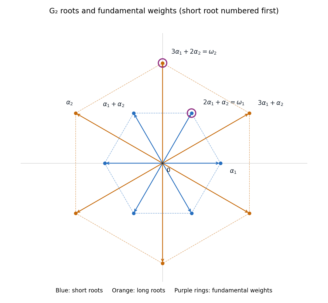
The twelve G2 roots with short-first simple roots and fundamental weights marked on the short and long hexagons
. Details. Let and . Relative to the simple coroots, the six positive coroots, in the root order above, have coordinatesFor example, has squared length one, so its coroot is ; the analogous length computation gives each other entry. Since , the pairings of with these coroots are , , , , , and . Their values at multiply to . The Weyl dimension formula therefore yields the G2 dimension polynomialThis holds for all nonnegative integers . In particular it gives dimensions and for and , and for . Reversing the numbering of the simple roots would interchange in the polynomial, so the short-first convention matters.
Past exam of the mathematics course of the University of Cambridge 2009 iii Paper 6 4 i Solution by Codex 0 Created 2026-10-03 Updated 2026-10-14
Codex 0 Created 2026-10-03 Updated 2026-10-14Let be a complex semisimple Lie algebra, choose a Cartan subalgebra and positive root system , and put . For a dominant integral weight , let be the finite-dimensional highest-weight representation with highest weight . The Weyl dimension formula isHere is the coroot, the pairing is between a weight and a coroot, and is the Weyl vector. The inner product can be any Weyl group invariant normalization on each simple factor: its scaling cancels from the ratios. The dominance condition means that is a nonnegative integer for each simple root.
Past exam of the mathematics course of the University of Cambridge 2009 iii Paper 6 3 iv Solution by Codex 0 Created 2026-10-03 Updated 2026-10-14
Codex 0 Created 2026-10-03 Updated 2026-10-14Use the ordered alphabetwith weights and . The crystal of the defining symplectic representation is the chainThe label of an arrow is its simple root color; a Kashiwara operator follows an arrow of color and lowers the weight by .
Here is a grid description of the entire tensor product of crystals, valid for every . Put one vertex at row and column , in the alphabet order above. Let be the set of chain positions with outgoing color , and the positions with incoming color :Their indicators are and . Use the crystal tensor-product ruleAn arrow is omitted if the selected factor has no outgoing arrow of that color. Thus the complete grid has a downward color- arrow when and , and a rightward color- arrow when and . There are no other arrows. These two coordinate rules specify every vertex and every edge of the requested general-rank drawing. The following figure displays the full grid at , including all components, together with the standard chain; increasing uses exactly the same grid construction.
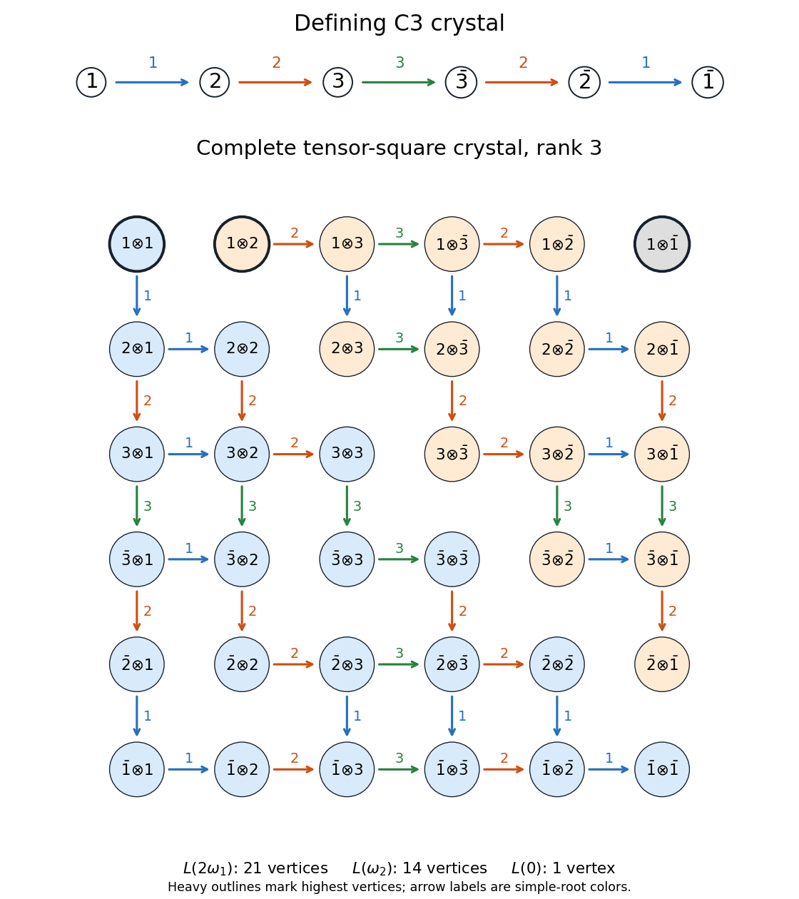
Defining C3 crystal and its complete tensor-square crystal with all colored arrows and the three highest-weight components
. Details. For completeness, highest vertices can be read from the raising rule, which selects the first factor when . If has an incoming edge of color , then ; either the raising operator acts nontrivially on , or and it acts nontrivially on . Thus a highest vertex must have . At , all vanish except . To be highest, the incoming color of , if any, must consequently be . For , the possibilities are exactlyTheir weights are , , and zero. Each occurs once. Connected highest-weight components of the crystal basis describe the irreducible representations in the tensor product of Lie algebra representations, soThis is the tensor-square decomposition of the defining symplectic representation. The symmetric square is ; the exterior square is the direct sum of its invariant inverse-form line and the primitive exterior square . Their dimensions are respectively , , and one, summing to . At , the chain has two vertices and the highest tensor vertices are only and : the decomposition is , of dimensions three and one.
Past exam of the mathematics course of the University of Cambridge 2009 iii Paper 6 3 iii Solution by Codex 0 Created 2026-10-03 Updated 2026-10-14
Codex 0 Created 2026-10-03 Updated 2026-10-14Identify the Cartan subalgebra with the coordinate space used above. The root reflection in any root of a root system fixes the perpendicular hyperplane. For every root of the Cn root system, its complete coordinate action isEvery unlisted coordinate is fixed, and changing the sign of the root leaves its reflection unchanged. These formulas follow directly from , with the coroot regarded as a vector of the Cartan subalgebra.
The Cn Weyl group is the signed symmetric group: its elements permute the coordinates and independently change their signs. The Weyl reflections associated with the simple roots interchange consecutive coordinates for and negate the last coordinate for . Thus
Past exam of the mathematics course of the University of Cambridge 2009 iii Paper 6 3 ii Solution by Codex 0 Created 2026-10-03 Updated 2026-10-14
Codex 0 Created 2026-10-03 Updated 2026-10-14Let be a four-dimensional symplectic vector space, with a symplectic basis . Its invariant inverse-form bivector may be chosen as . Put , so . Define a symmetric bilinear form on the six-dimensional exterior square byIt is symmetric because both factors have degree two. It is nondegenerate: in the six-element wedge basis, every pairs nontrivially with the wedge of the complementary pair and with no other basis vector. Since , the orthogonal complementhas dimension five and inherits a nondegenerate bilinear form. It is the primitive exterior square, equivalently the kernel of the symplectic contraction of an exterior square.
The symplectic Lie algebra preserves . It also preserves , since its elements have trace zero and the induced action on is multiplication by that trace. The exterior-power Lie algebra representation therefore preserves and , giving a Lie algebra homomorphismTo show injectivity, suppose acts as zero on . It already acts as zero on the invariant line , so it kills all of . For any basis , this meansIf , choose distinct from ; the coefficient of forces . Thus is diagonal. The same identity gives for every pair. Applying this to three distinct indices forces each diagonal entry to vanish. Hence and is injective.
Finally and . Injectivity between these equal-dimensional vector spaces gives surjectivity. Every nondegenerate complex symmetric bilinear form on a five-dimensional space is equivalent to the standard one. We have therefore constructed the exceptional isomorphism between sp4 and so5:
Past exam of the mathematics course of the University of Cambridge 2009 iii Paper 6 3 i Solution by Codex 0 Created 2026-10-03 Updated 2026-10-14
Codex 0 Created 2026-10-03 Updated 2026-10-14Write , and let denote a matrix unit. The diagonal Cartan subalgebra consists ofFor a diagonal matrix, . Substituting into the symplectic relation shows that the following are root vectors:The zero weight space is spanned by . The symplectic equation pairs the remaining entries exactly as in this table; the displayed vectors and the are independent and span the algebra. This proves the root-space decompositionThere are roots of a root system, each with one-dimensional root space, giving .
The upper triangular root vectors select preciselyThe simple roots of this Cn root system areIndeed, the positive roots of a root system have expansionsThese expansions also identify the highest root:Normalize the coordinate inner product by . The simple coroots are for and . Solving gives the fundamental weightsIn the sum of the positive roots of a root system, the pair contributes , and the long root contributes another . Therefore the Weyl vector isThese are the Positive-root data for Cn.
For , the finite Dynkin diagram is a chain of vertices. The bonds between and for are single. The last bond is double, with its arrow pointing from the long root toward the short root . For the Extended Dynkin diagram, add at the other end, doubly bonded to , with arrow toward . The following Cn Dynkin diagrams include both ends and the low-rank cases.
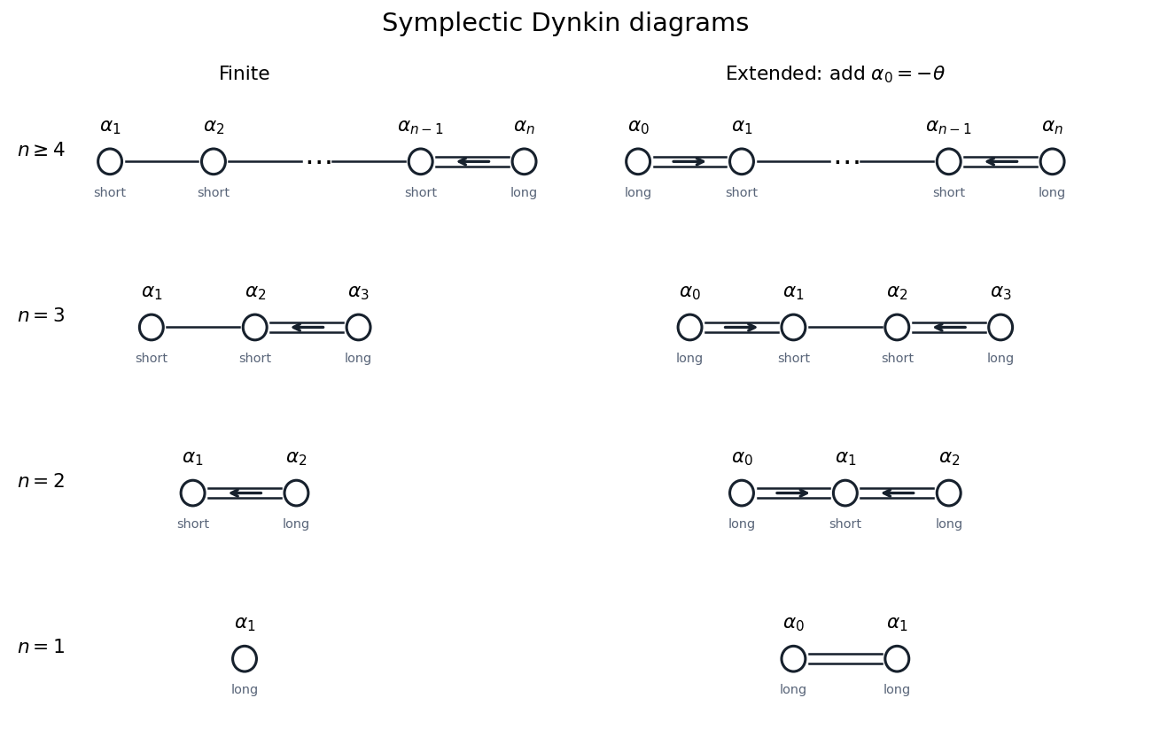
Finite and extended Cn Dynkin diagrams with arrows toward the short roots and separate rank-one and rank-two cases
. Details. At , there is just the root and one finite vertex. The affine Cartan matrix is ; its two vertices have equal root length, so the double bond has no arrow.
Past exam of the mathematics course of the University of Cambridge 2009 iii Paper 6 1 ii Solution by Codex 0 Created 2026-10-03 Updated 2026-10-14
Codex 0 Created 2026-10-03 Updated 2026-10-14The derived series of a Lie algebra isThe algebra is a solvable Lie algebra if for some . Here a bracket of subspaces means the linear span of their Lie brackets.
The Lie theorem states that a nonzero finite-dimensional representation of a complex solvable Lie algebra has a common eigenvector; equivalently, its operators can be simultaneously upper triangularized. Applied to an Irreducible Lie algebra representation, the common eigenvector gives a nonzero invariant line, which must be the entire module. A scalar action respects the Lie bracket exactly when . Thus, in the finite-dimensional setting,Every functional displayed gives a one-dimensional irreducible, and two such modules are isomorphic exactly when their functionals agree.
The finite-dimensional qualification is essential here, although the printed wording does not repeat it. For example, let and act on by and . These operators satisfy . A nonzero submodule stable under is an ideal . Stability under forces , so the two polynomials, having the same degree and leading coefficient, are equal. In characteristic zero a polynomial invariant under a nonzero shift is constant. The module is therefore an infinite-dimensional simple module for the two-dimensional affine Lie algebra. It rules out extending the one-dimensional classification to unrestricted representations.
Past exam of the mathematics course of the University of Cambridge 2009 iii Paper 6 1 i Solution by Codex 0 Created 2026-10-03 Updated 2026-10-14
Codex 0 Created 2026-10-03 Updated 2026-10-14First consider finite-dimensional Lie algebra representations. The operators representing an abelian Lie algebra commute. They have a common eigenvector: take an eigenspace for the first operator of a basis of the algebra, observe that every remaining operator preserves it, and repeat inside this nonzero space. The resulting line is an invariant subspace, so an irreducible representation must be one-dimensional. Its action has the form for a linear functional . Conversely, every such functional defines a Lie algebra representation, since both the Lie brackets in the algebra and the commutators of its scalar operators vanish. Distinct functionals give nonisomorphic representations. Thus the irreducibles are precisely the characters .
Even without a finite-dimensional assumption on the module, this conclusion for a finite-dimensional abelian Lie algebra follows from the Weak Hilbert Nullstellensatz: its universal enveloping algebra is the polynomial algebra . A simple module over a commutative algebra is its quotient by a maximal ideal, and every maximal ideal of this polynomial algebra over has residue field .
Indecomposable does not imply irreducible. For the one-dimensional abelian Lie algebra , let act on by the Nilpotent Jordan blockThe line spanned by the first coordinate vector is an invariant subspace, so the module is reducible. If it were a direct sum of two nonzero submodules, both would have dimension one; nilpotence would force to act as zero on both, contrary to . Thus it is an indecomposable representation.
For a finite-dimensional module , put and define its generalized weight spaces intrinsically byTo obtain the decomposition, choose a basis of , split into generalized eigenspaces of , and successively split each piece by . All the pieces are submodules because the acting operators commute. On one resulting piece, has a unique eigenvalue . The commuting operators can be simultaneously upper triangularized by repeating the common-eigenvector argument on quotients. Hence on this piece every is strictly upper triangular. Any linear combination is also strictly upper triangular, and its th power vanishes. Extending linearly therefore identifies the piece with . Different tuples give disjoint pieces; if a component has a different tuple from , at least one is invertible there. Consequentlywith only finitely many nonzero summands. Since the definition uses every rather than a chosen basis, this generalized-weight decomposition for a nilpotent Lie algebra is canonical. Its summands need not be irreducible, as the Jordan block example already shows.
Past exam of the mathematics course of the University of Cambridge 2009 iii Paper 59 3 d Solution by Codex 0 Created 2026-10-03 Updated 2026-10-14
Codex 0 Created 2026-10-03 Updated 2026-10-14Because is projective twistor space, the printed column represents the line , not a distinguished nonzero vector. Its stabilizer subgroup consists of matrices whose first column is a nonzero multiple of :The block form is necessary to preserve the line, and conversely every such determinant-one matrix preserves it. By transitivity, the orbit map is onto . Its two values agree precisely when , equivalently when . This gives the homogeneous space identificationThe dimensions also agree: , while the free and parameters give ; the quotient has dimension three.
This coset space is not a quotient group, because is not a normal subgroup. For example . Let have upper-left block and identity on the other two coordinates. Then but sends to , so it is not in . Thus multiplying coset representatives does not define a well-defined group operation.
If instead one required the literal vector to be fixed, one would have and ; its quotient would be , not . The projective reading is required by the printed target quotient and the flag manifold definition.
Past exam of the mathematics course of the University of Cambridge 2009 iii Paper 59 3 c Solution by Codex 0 Created 2026-10-03 Updated 2026-10-14
Codex 0 Created 2026-10-03 Updated 2026-10-14The special linear group acts on the twistor correspondence by . Since an invertible linear map preserves inclusion, this is again an incident flag. The two projections commute with that action:This is precisely equivariance: projecting a transformed flag gives the same result as transforming its projection. In particular sends the twistor line of a spacetime point to the line of the transformed point and sends the alpha-plane of a twistor to that of its transformed twistor. The incidence geometry is preserved, even when a transformation takes a point out of the chosen affine Minkowski chart.
Pinned article: Introduction to the OurBigBook Project
Welcome to the OurBigBook Project! Our goal is to create the perfect publishing platform for STEM subjects, and get university-level students to write the best free STEM tutorials ever.
Everyone is welcome to create an account and play with the site: ourbigbook.com/go/register. We belive that students themselves can write amazing tutorials, but teachers are welcome too. You can write about anything you want, it doesn't have to be STEM or even educational. Silly test content is very welcome and you won't be penalized in any way. Just keep it legal!
Intro to OurBigBook
. Source. We have two killer features:
- topics: topics group articles by different users with the same title, e.g. here is the topic for the "Fundamental Theorem of Calculus" ourbigbook.com/go/topic/fundamental-theorem-of-calculusArticles of different users are sorted by upvote within each article page. This feature is a bit like:
- a Wikipedia where each user can have their own version of each article
- a Q&A website like Stack Overflow, where multiple people can give their views on a given topic, and the best ones are sorted by upvote. Except you don't need to wait for someone to ask first, and any topic goes, no matter how narrow or broad
This feature makes it possible for readers to find better explanations of any topic created by other writers. And it allows writers to create an explanation in a place that readers might actually find it.
Figure 1. Screenshot of the "Derivative" topic page. View it live at: ourbigbook.com/go/topic/derivativeVideo 2. OurBigBook Web topics demo. Source. - local editing: you can store all your personal knowledge base content locally in a plaintext markup format that can be edited locally and published either:This way you can be sure that even if OurBigBook.com were to go down one day (which we have no plans to do as it is quite cheap to host!), your content will still be perfectly readable as a static site.
- to OurBigBook.com to get awesome multi-user features like topics and likes
- as HTML files to a static website, which you can host yourself for free on many external providers like GitHub Pages, and remain in full control

Figure 2. You can publish local OurBigBook lightweight markup files to either OurBigBook.com or as a static website.
Figure 3. Visual Studio Code extension installation.
Figure 5. . You can also edit articles on the Web editor without installing anything locally. Video 3. Edit locally and publish demo. Source. This shows editing OurBigBook Markup and publishing it using the Visual Studio Code extension. 
- Infinitely deep tables of contents:




All our software is open source and hosted at: github.com/ourbigbook/ourbigbook
Further documentation can be found at: docs.ourbigbook.com
Feel free to reach our to us for any help or suggestions: docs.ourbigbook.com/#contact