
The Cantor set is obtained from by repeatedly deleting the open middle third of every remaining interval. Its first stages retain , then four intervals of length , then eight of length . After level , there are retained intervals of length . The Cantor set is the intersection of all these stages, rather than the set of endpoints visible in any finite drawing.
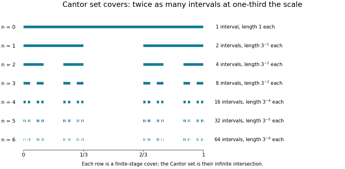
Finite stages of the Cantor construction supply covers at successively smaller scales
. Details. Equivalently,Thus its points admit a base-three expansion using only zero and two. The word “admit” handles numbers with two expansions: is retained as an endpoint. Every infinite binary choice determines a point of , and differing choices give differing points, so is uncountable.
Its total retained interval length is , so has zero Lebesgue measure. It is nevertheless nonempty, compact, and uncountable, and has Hausdorff dimension : the covers and mass bounds are worked out in Hausdorff dimension of the Cantor set. This separates counting, ordinary length, and fine-scale geometric size in one concrete example.
The self-similarity is exact:The Cantor distribution puts half the probability into each copy at every split. It has a continuous cumulative distribution function, the Cantor function, while all its mass lies on a Lebesgue null set. This makes the construction useful in measure theory as well as fractal geometry: it provides a concrete model in which several plausible meanings of “small” disagree.


The Cantor set is a classic example of a set that is uncountably infinite, has zero measure, and exhibits some counterintuitive properties in terms of size and density. It is constructed through an iterative process starting with the closed interval \([0, 1]\). Here’s how the construction works: 1. **Start with the interval**: Begin with the closed interval \([0, 1]\).
New to topics? Read the docs here!