The cumulative distribution function of a real random variable isIt records the probability accumulated up to a threshold. It is a nondecreasing function and is right-continuous; its limits are zero at and one at . These properties follow from ordered threshold events, continuity from above of a measure, and continuity from below of a measure. A cumulative distribution function determines the entire probability distribution on the real line. [ref].
For ,where is its left-hand limit. The second formula measures a jump. Thus ; changing an endpoint is harmless only when its point probability is zero.
For the finite example under probability distribution, is below zero, on , on , and on . In particular , but , so the jump gives . For the density example, on , and its increase from to is .
When an absolutely continuous probability distribution has probability density function , its cumulative distribution function is and almost everywhere. A continuous cumulative distribution function by itself does not guarantee such a density: the Cantor distribution is an important exception.
If a random variable takes values in , its cumulative distribution function satisfiesIndeed for every outcome. Taking expected values and using Tonelli's theorem proves the formula, including when the probability distribution has atoms. For a probability density function , the same proof reverses the order in . Thus , restricted to , is a probability density function whenever . The reflected construction using has normalising constant and is closely related to an integrated tail distribution.
For , every difference quotient at is nonnegative and bounded by . The spherical derivative of a singular measure vanishes, so the two-sided derivative is zero Lebesgue almost everywhere. A singular distribution function need not be constant: differentiation almost everywhere does not recover increments without absolute continuity of a function of the function.
The Kolmogorov distance between two probability distributions with cumulative distribution functions is .
If a cumulative distribution function is constant between consecutive lattice points spaced by near zero, then its Kolmogorov distance from the standard normal distribution function is at least half the increase of that function across one such interval. This gives a lower bound of order .
If has a continuous cumulative distribution function , then has the uniform distribution on . Combined with inverse transform sampling, this constructs the monotone rearrangement to a target with quantile function .
For correct continuous conditional forecasts, the conditional probability integral transform is uniform given the entire past. Iterating conditional probabilities makes the transformed sequence independent and uniform. Uniformity and serial checks assess absolute predictive calibration using only the forecast distributions and observations.
If distribution functions converge pointwise to a continuous distribution function , then the convergence is uniform. Choose finitely many points whose successive -increments and two tails are small, then use monotonicity to squeeze between its values at adjacent points.
The empirical distribution function counts the fraction of observations at or below a threshold. For a statistical sample of real observations , defineEach indicator function contributes one exactly when its observation is counted. Equivalently, , where the empirical measure assigns probability mass to each observation, including repeated observations.[ref]
Choose the illustrative statistical sample . Its empirical distribution function isFor example, counts both observations equal to , , and . There is no observation at , so there is no jump there. The five observations produce only four distinct jump locations.
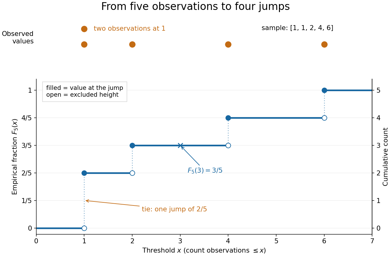
The convention makes the empirical distribution function right-continuous: once a threshold reaches an observation, that observation remains counted immediately to its right. For a finite statistical sample, the count is constant from any up to the next larger observed value, proving right continuity. Its left-hand limit counts observations strictly below , soA value occurring times causes one jump of size . At the jump is ; at , , and each jump is . All jumps sum to one. Thus the empirical distribution function is a nondecreasing step function with limits zero and one, and is itself a valid cumulative distribution function.
This turns many questions about data into simple cumulative distribution function operations. The observed fraction in is : for it is , counting and but excluding both s. Including the left endpoint gives . A sample quantile reads the same staircase in reverse: the smallest threshold reaching is . Unlike a histogram, this representation requires no choice of bins; its jumps retain every observation and its multiplicity.
The exact description of a finite statistical sample must be distinguished from a statistical model for how it was obtained. The empirical distribution function is defined for any finite list, with no independence assumption. Once the list is observed, its counts are fixed. For statistical inference, one often models as independent and identically distributed random variables with an unknown population cumulative distribution function . Then describes the sampling law, while varies across repeated statistical samples. The value is an observed fraction and an estimate of ; it does not establish that the population probability is . Even when is continuous, every finite is discrete.
For any threshold fixed before sampling, the indicator functions are independent Bernoulli random variables with success probability . Therefore the count has a binomial distribution andThe expected value follows by adding the expected values of the indicator functions; the variance follows by adding their variances using independence and dividing by . Thus is an unbiased estimator of at a fixed threshold. Controlling the error at every threshold at once requires more than a fixed-threshold calculation: the DKW inequality supplies such control, and the Glivenko-Cantelli theorem describes its uniform convergence almost surely as grows.
Comparing with a proposed cumulative distribution function also motivates goodness-of-fit tests, including the Kolmogorov-Smirnov test, the Anderson–Darling test, and the Cramér–von Mises criterion. A standard Kolmogorov-Smirnov test calibration assumes a fully specified continuous population law; fitting its statistical parameters from the same statistical sample changes that calibration.[ref]
1.3.5.16. Kolmogorov-Smirnov Goodness-of-Fit Test. NIST and SEMATECH e-Handbook of Statistical Methods; Characteristics and Limitations, items 1 and 3; Definition, test statistic and fully specified distribution requirement
For independent and identically distributed real random variables with cumulative distribution function , the Dvoretzky-Kiefer-Wolfowitz inequality gives, for every and ,The supremum is the Kolmogorov distance: a single event controls all thresholds simultaneously. The bound holds for discrete, continuous, and mixed probability distributions.[ref]
For one fixed threshold, Hoeffding's inequality gives the same expression as an upper bound on . That fixed-threshold result alone does not justify moving the supremum inside the probability. The DKW inequality is the stronger statement needed for a simultaneous empirical distribution confidence band.
Fix a failure probability and assume an independent and identically distributed statistical sample. A finite-sample confidence band for its population cumulative distribution function isHere is the natural logarithm. The DKW inequality impliesThis is simultaneous coverage over the whole real line, valid at each fixed sample size.[ref]
To obtain the band, solve for the positive . Outside a failure event of probability at most , for every . Since a cumulative distribution function already lies in , clipping the endpoints to this interval preserves the coverage event. The guarantee is at least , and need not equal it.
Choose , giving at least simultaneous coverage under the stated model. For , respectively, the half-widths before clipping areFor the chosen five observations, the band at is , while at it is approximately . At the unclipped band would be , so clipping gives . The broad uncertainty is informative: five observations give a precise description of themselves, but a coarse bound for an unknown population cumulative distribution function.
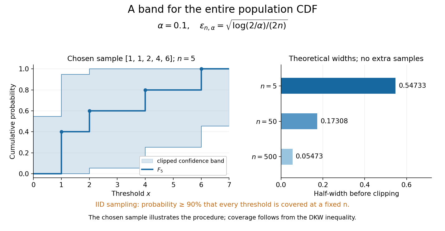
Finite-sample simultaneous uncertainty around an empirical distribution function
. Left: the chosen five observations give and its band clipped to , using . Right: theoretical half-widths for , with no additional samples constructed. The confidence band has coverage at least under independent and identically distributed sampling; the drawing illustrates the procedure and does not establish its coverage. Details.A collection of pointwise confidence intervals only promises coverage separately at each preselected threshold; it does not promise coverage of an entire cumulative distribution function. Here the one simultaneous event permits inspecting any threshold after seeing the data. The probability refers to repeated sampling of the entire statistical sample, with fixed. It does not assign probability to a fixed after observing this particular band, and it is not a prediction interval for a future observation. The displayed comparison gives a guarantee for each fixed separately, not simultaneous validity over all sample sizes or an optional stopping rule. The chosen observations are an illustration; the coverage claim follows from the DKW inequality, not from their appearance or a simulation. Dependence or observations with different sampling laws require another argument.
At fixed , multiplying by divides the half-width by . Conversely, a desired half-width is ensured by , rounded up to an integer. For and , this sufficient sample size is . This makes the confidence band useful for planning how many observations are needed before estimating threshold probabilities to a chosen simultaneous accuracy.
The test rejects for large values of this tail-weighted empirical discrepancy. For a specified continuous null, its standard limiting statistic is , using a Brownian bridge. The reciprocal variance weight gives tail deviations more influence than the Cramér–von Mises criterion. If null parameters are estimated, fitting must be included when computing or simulating its reference law.
This goodness-of-fit criterion integrates the squared difference between the empirical distribution function and a specified continuous null distribution. Under a fully specified null, the probability integral transform makes its law distribution-free; its limiting law is for a Brownian bridge. Parameter fitting changes that calibration.
The empirical distribution process is the centred, scaled empirical distribution function of an independent sample with cumulative distribution function . Its mean is zero and its covariance is . This follows by expanding the two indicator averages: different sample indices have zero covariance, while the same index contributes the covariance of the two nested events. The scaling by keeps these covariances independent of .
For an independent sample with cumulative distribution function , the empirical distribution process converges in the supremum norm on to the F-Brownian bridge. The convergence uses outer expectation and inner expectation when finite-sample Borel measurability fails. It is a full function-space theorem, stronger than the Finite-dimensional Brownian bridge limit of an empirical distribution process. No continuity of is required. The continuous mapping theorem gives convergence of the supremum statistic; for continuous , its range contains and the bridge vanishes at zero and one, giving the Kolmogorov-Smirnov theorem. The function-space statement is stated here as a theorem; its tightness assertion is an additional ingredient beyond the finite-dimensional covariance calculation.
For fixed , the vector converges in distribution to , where is a standard Brownian bridge. To prove it, write the vector as times the sum of independent centred bounded indicator vectors. Their covariance matrix is . The multivariate central limit theorem gives a centred multivariate normal distribution with this covariance, exactly the bridge vector. Singular covariance matrices, including endpoint times or repeated values of , cause no problem. This is a finite-dimensional assertion; a full function-space limit additionally requires tightness.