 Histogram

A histogram groups numerical observations into adjacent intervals called bins and draws one rectangle per bin. Its attraction is that a long list of values becomes a visible pattern of concentration, gaps and skewness. Specify the bin edges, the treatment of values on those edges, and what the vertical axis means: count, proportion, or density. Those choices are part of the graphic. ^[ref]

Let $n>0$ observations be covered by disjoint bins $B_j$ with positive widths ${\Delta }_j$ and counts $n_j$, so ${\sum }_j{n}_j=n$. For example, use left-closed, right-open bins, closing the final right edge too. The three common height choices have different meanings:

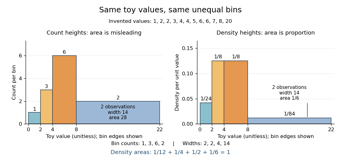
For the density convention, a histogram is a piecewise constant probability density function estimate:Its normalization follows by adding rectangular areas:If the observations have units, density has reciprocal units; a density height is not a probability and can exceed $1$. With equal bin widths, count heights and density heights differ only by a common scale factor. With unequal widths, count-height areas $n_j{\Delta }_j$ give wider bins extra visual weight unrelated to their counts. Dividing by width removes that distortion. R's histogram documentation explicitly describes area-one normalization for unequal bins. ^[ref]

Reuse the twelve invented values under box plot, with bins $[0,2),[2,4),[4,8),[8,22]$. The counts are $(1,3,6,2)$ and the widths are $(2,2,4,14)$. Hence the density heights and areas are exactlyThe second and third bars have equal density heights even though the third contains twice as many observations: it is also twice as wide. The last bar contains only two observations; its count-height area would be $2\cdot 14=28$, larger than the six-observation bar's $6\cdot 4=24$. Its correct density area is only $1/6$.

Bin choice trades detail against stability. Broad bins merge distinctions: the toy bin $[8,22]$ hides the empty stretch between $8$ and $20$. Narrow bins expose gaps but can make each individual observation dominate a bar. With one-unit bins starting at $0$, the bins $[2,3),[4,5),[6,7)$ each contain two values and appear equally prominent; that apparent pattern depends on grouping the repeated integers together. Moving the bin origin also changes membership without changing the observations. For density estimation, this is a form of the bias-variance tradeoff: averaging over broad bins loses local detail, while narrow bins give more variable density estimates across repeated statistical samples. ^[ref] A useful practice is to compare a few plausible widths and offsets, keeping common edges when comparing groups. Automatic bin selectors are starting points, rather than guarantees of a unique correct picture. ^[ref]

A histogram retains only bin membership. Its density estimate spreads each bin's fraction uniformly across that bin, so our last bar assigns density throughout $[8,22]$ even though the only toy values there are $8$ and $20$. It does not recover within-bin positions or observation order, and a visually convincing shape does not establish a population probability distribution. A box plot provides a complementary compact summary of quartiles; neither graphic replaces the original observations.