Probability distribution ( $μ_{X} (B) = P (X \in B)$ )

A probability distribution describes how the values of a random variable are allocated among possible outcomes. More precisely, the law of a random variable

X

assigns each measurable set

B

the probability

μ_{X} (B) = P (X \in B) .

(1)

It is a probability measure on the values of

X

. The underlying experiment can be more elaborate than the output: different experiments may produce the same probability distribution. The law of a random variable retains the probabilities needed to answer questions about that output. ^[ref].

For a finite example, let

X

take values

0, 1, 3

with probability mass function

p_{X} (0) = 0.2

p_{X} (1) = 0.5

p_{X} (3) = 0.3

. Its probabilities sum to one. The event

0 < X \leq 1

has probability

0.5

, whereas

0 \leq X \leq 1

has probability

0.7

: including one endpoint matters when it carries positive probability.

For a contrasting random variable

Y

, choose the probability density function

f_{Y} (y) = 2 y

0 \leq y \leq 1

, and zero elsewhere. It integrates to one. Now

P (1/4 < Y \leq 3/4) = \int_{1/4}^{3/4} 2 y d y = 1/2

, while every single outcome has probability zero. The probability density function can have height

f_{Y} (0.8) = 1.6

: probabilities come from integrals over outcome ranges.

Figure 1.
Probability masses and densities accumulate into cumulative distribution functions
. Left: $X$ takes values $0, 1, 3$ with probability masses $0.2, 0.5, 0.3$ , so its cumulative distribution function jumps at those values; open and filled markers show the excluded and included heights at a jump. Right: $Y$ has probability density function $2 y$ on the interval $[0, 1]$ and cumulative distribution function $y^{2}$ there. The shaded integral over $(1/4, 3/4]$ and the corresponding cumulative distribution function increase both equal $1/2$ . **Details**.

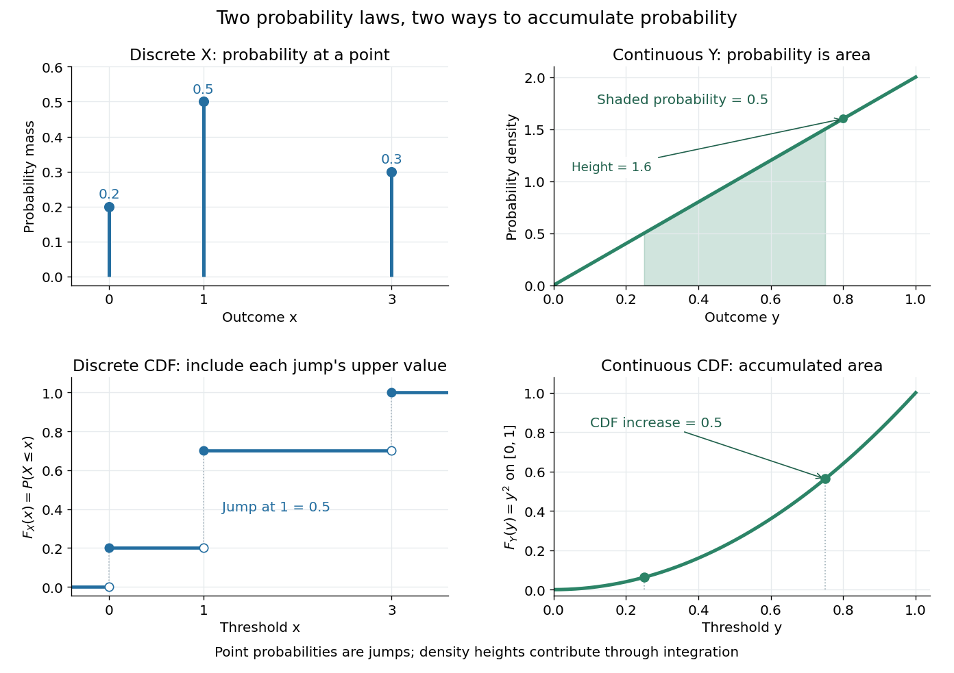
The cumulative distribution function answers all threshold questions for a real random variable, regardless of whether there are jumps or a probability density function. A quantile function reverses the direction of the question: given a cumulative probability level, find a threshold. This connects descriptive summaries to inverse transform sampling, which constructs a chosen probability distribution from a uniform distribution.

Table of contents

Probability vector ( $p_{i} \geq 0, \sum_{i} p_{i} = 1$ )

 1  0

A probability vector lists the probabilities of the outcomes in a finite sample space. Its entries are nonnegative and sum to one, so a column probability vector is a point of a probability simplex. Row and column conventions describe the same probability distribution, but they determine whether a stochastic matrix acts on the right or its transpose acts on the left.

Finite probability distribution ( $p \geq 0, \sum_{x} p (x) = 1$ )

 0  0

A probability mass function with finite positive-mass support, nonnegative masses and total mass one. Listing its support means listing exactly positive-mass outcomes once, excluding zero-probability endpoint outcomes. A computational interface returning floating-point masses generally approximates exact rational or real probabilities.

Product of finite probability distributions ( $p (x, y) = p_{1} (x) p_{2} (y)$ )

 0  0

Given two finite probability distributions, assign the product of their probability masses to each ordered pair. The support is the Cartesian product of the two positive-mass supports. Distributivity gives

\sum_{x, y} p_{1} (x) p_{2} (y) = (\sum_{x} p_{1} (x)) (\sum_{y} p_{2} (y)) = 1

. This is the joint distribution for independent coordinate outcomes; it is a construction from the marginals, not a claim that arbitrary jointly observed coordinates are independent.

Empirical probability distribution ( $p (x) = n^{- 1} \sum_{i = 1}^{n} 1_{{x_{i} = x}}$ )

 0  0

For a nonempty finite sample, assign each distinct observed value its relative frequency. The observed values form the finite positive-mass support; the counts sum to the sample size, so the probabilities sum to one. Repeated observations increase the same outcome's mass rather than adding repeated support entries.

Pushforward of a finite probability distribution ( $q (y) = \sum_{x : f (x) = y} p (x)$ )

 0  0

For a finite probability distribution

p

with support

S

and a total function

f : S \to Y

, assign each image value the combined mass of its preimages. Its support is exactly the finite image

f (S)

, listed without repetitions. Every listed mass is positive because it contains at least one positive source mass.

The fiber of a function construction gives a set partition of

S

, so finite summation gives

\sum_{y} q (y) = \sum_{x \in S} p (x) = 1

. This proves nonnegativity and normalization without assuming that

f

is injective. In code, mapping support values and then overwriting repeated image keys is incorrect; repeated keys must have their masses added. For example, mapping a uniform distribution on four consecutive integers to parity produces two outcomes with mass one half each.

Waiting-time distribution ( $p (t) = - S^{'} (t)$ )

 0  0

The probability distribution of a nonnegative duration until an event. For a continuous duration with survival function

S (t) = P (T > t)

, its probability density function is

p (t) = - S^{'} (t)

. A constant hazard gives an exponential distribution; successive independent first-order waits give a convolution, as in the two-step catalytic waiting time.

Two-step catalytic waiting time ( $p (t) = \frac{k _{a} k _{b}}{k _{a} - k _{b}} (e^{- k_{b} t} - e^{- k_{a} t})$ )

 0  0

The convolution of two independent sequential exponential waiting times has the displayed normalized density and mean

k_{a}^{- 1} + k_{b}^{- 1}

. At equal rates its limit is

k^{2} t e^{- k t}

. A measured density of this form supports a multistep kinetic mechanism without uniquely identifying its hidden chemical intermediates.

Self-decomposable distribution ( $X = d c X + R_{c}, R_{c} ⊥ X$ )

 0  0

A probability distribution is self-decomposable if, for every

0 < c < 1

, an independent remainder

R_{c}

can be chosen so that the displayed equality in distribution holds. A normal distribution

N (μ, σ^{2})

admits a normal distribution remainder with mean

(1 - c) μ

and variance

(1 - c^{2}) σ^{2}

. For an exponential distribution of rate

λ

, choose

R_{c} = 0

with probability

c

and otherwise an independent exponential distribution of rate

λ

. Its moment-generating function is

c + (1 - c) λ / (λ - t) = (λ - c t) / (λ - t)

; multiplication by

M_{X} (c t)

proves the claim using the uniqueness theorem for moment-generating functions.

Normalization of a probability distribution ( $\int f (x) d x = 1$ )

 0  0

A probability distribution assigns total probability one to its sample space. For a nonnegative probability density function this means that its integral over the full domain equals one; for a probability mass function the sum of its masses equals one. A nonnegative integrable function with positive finite integral can be divided by that integral to normalize it. A negative function cannot be a probability density function even if a formal manipulation purports to normalize it.

Mixed probability distribution ( $μ = α μ_{d} + (1 - α) μ_{c}$ )

 0  0

A mixed probability distribution combines a discrete probability distribution with a continuous probability distribution. For example, put probability

1/4

at zero and probability

3/4

into a uniform distribution on

(0, 1)

. Its cumulative distribution function is

0

for

x < 0

1/4 + 3 x /4

for

0 \leq x < 1

, and

1

for

x \geq 1

. The jump at zero and the continuous increase both contribute; neither an ordinary probability density function alone nor a probability mass function alone describes the whole law.

Mixture of a point mass and an exponential distribution ( $L (Y) = p δ_{- c} + (1 - p) Exp (λ)$ )

 0  0

Let

c > 0

0 \leq p \leq 1

and

λ > 0

. With probability

p

, take

Y = - c

; otherwise draw an exponential distribution of rate

λ

. This mixed probability distribution has a negative atom and a continuous nonnegative component. Its moments are

E [Y] = - p c + (1 - p) / λ

and

E [Y^{2}] = p c^{2} + 2 (1 - p) / λ^{2}

. The law of total variance equivalently gives

Var (Y) = (1 - p) / λ^{2} + p (1 - p) (c + 1/ λ)^{2}

When

p < 1

, conditioning on

Y \geq 0

selects exactly the exponential component, so

P (Y \geq t ∣ Y \geq 0) = e^{- λ t}

for

t \geq 0

. An ordinary probability density function for the continuous component integrates to

1 - p

, not one; the missing mass is the atom, not a normalization error.

Uniform distribution with an atom at zero ( $L (S) = (1 - q) δ_{0} + q Unif (0, r)$ )

 0  0

For

0 \leq q \leq 1

and

r > 0

, this mixed probability distribution has probability mass

1 - q

at zero and ordinary probability density function

q / r

(0, r)

. That ordinary density integrates to

q

, not to one; conditioned on

S > 0

, the law is the uniform distribution on

(0, r)

. Its cumulative distribution function is zero for

s < 0

1 - q + q s / r

for

0 \leq s < r

, and one for

s \geq r

For each positive integer

k

, integration gives

E [S^{k}] = q r^{k} / (k + 1)

. Thus the expected value is

q r /2

and the variance is

q r^{2} /3 - q^{2} r^{2} /4

. The nonzero atom contributes to normalization even though it contributes zero to positive moments. At

q = 0

, conditioning on positive delay is undefined because the conditioning event has probability zero.

Probability mass ( $P (X = x)$ )

 0  0

The probability mass at an outcome

x

is the probability of its singleton,

P (X = x)

. It equals the jump

F_{X} (x) - F_{X} (x^{-})

of the cumulative distribution function. For a discrete probability distribution these masses form the probability mass function; a continuous probability distribution gives every individual outcome mass zero. Positive probability mass at a point is distinct from the height of a probability density function.

Heavy-tailed distribution ( $E e^{θX} = \infty (θ > 0)$ )

 1  0

In the right-tail convention, every positive exponential moment is infinite. This is a tail property, not the assertion that the variance or all power moments must be infinite. A heavy-tailed subexponential distribution has the additional property that a sum's far tail is dominated by one large summand.

Subexponential distribution (heavy-tailed, $P (X_{1} + X_{2} > x) \sim 2 P (X_{1} > x)$ )

 0  0

For nonnegative independent and identically distributed random variables with unbounded support, this is the displayed two-summand tail asymptotic. The probability that the maximum exceeds

x

1 - F (x)^{2} \sim 2 \overline{F} (x)

, so the sum and maximum have asymptotically the same tail. This is the basic single-large-arrival effect relevant to queue overflow. The concentration-theory sub-exponential random variable uses a separate light-tail convention.

Infinite divisibility (probability, $μ = μ_{n}^{* n} for every n \geq 1$ )

 0  0

A probability distribution is infinitely divisible if, for every positive integer

n

, it is the distribution of a sum of

n

independent and identically distributed random variables. Their common distribution may depend on

n

. A normal distribution has this property by dividing its mean and variance by

n

; a Poisson distribution has it by dividing its rate. The unit-time law of a Lévy process is infinitely divisible because it is the sum of its increments on

n

equal time intervals.

Predictive distribution

 0  0

A probability law for a future observation conditional on currently available information. A posterior predictive distribution integrates the observation model over the posterior distribution of unknown parameters; a plug-in predictive law instead fixes an estimate of those parameters.

Predictive variance ( $Var (Y_{*} ∣ D)$ )

 0  0

The variance of a predictive distribution quantifies spread of a future quantity conditional on the observed data and model assumptions. For a noisy future observation

Y_{*} = f_{*} + ϵ_{*}

with fresh independent noise of variance

σ^{2}

, it is

Var (f_{*} ∣ D) + σ^{2}

. It should therefore be distinguished from the latent-function posterior variance.

Non-degenerate probability distribution

 0  0

A probability distribution is non-degenerate when it is not a point mass. This condition excludes constant limits in limit theorems and in the maximum domain of attraction of a distribution function.

Support of a probability distribution ( $supp μ = {x : μ (U) > 0 for every open U ∋ x}$ )

 0  0

For a probability measure on a topological space, its support consists of the points whose every open neighborhood has positive probability. For a continuous effort distribution supported on an interval, every open subinterval of that interval has positive probability.

Full-support probability distribution on a finite alphabet ( $supp (p) = X$ )

 0  0

A probability mass function

p

has full support on a specified finite alphabet if

p_{x} > 0

for every symbol in that alphabet. This is relative to the chosen alphabet: deleting zero-probability symbols produces a smaller alphabet on which the same law has full support. In a weighted prefix code problem, full support makes every shortening of a retained codeword strictly reduce expected codeword length. Without it, a minimum-cost code tree may contain redundant zero-weight branches.

Effort support

 0  0

An effort support is the support of a probability distribution used to randomize effort in a contest. The all-pay indifference equation with random entry determines this support together with its distribution function.

Kurtosis ( $κ = E [(X - E X)^{4}] / Var (X)^{2}$ )

 1  0

For a real random variable

X

with mean

μ = E X

, finite positive variance

0 < σ^{2} = Var (X) < \infty

, and finite fourth moment, kurtosis is the fourth central moment divided by the square of the variance:

κ (X) = \frac{E [( X - μ ) ^{4} ]}{σ ^{4}} = E [Z^{4}], Z = \frac{X - μ}{σ} .

(1)

The standard score

Z

measures distance from the mean in standard deviations. Its fourth power gives a value ten standard deviations away a weight

1 0^{4} = 10000

inside the expected value. Thus a small probability mass far from the mean can strongly affect kurtosis. It is useful for describing the contribution of extreme standard scores, but does not by itself describe the height or shape of a probability density function near its peak.^[ref]

The normal distribution has kurtosis

3

. A random scale can increase kurtosis even when the conditional distribution is normal. A constant random variable has zero variance, so this ratio is undefined. If the variance is finite and positive but the fourth central moment is infinite, the ratio can be written

+ \infty

in an extended sense; it is not a finite kurtosis. If the variance itself is infinite or the mean is undefined, the displayed normalization is unavailable.

Excess kurtosis ( $γ_{2} = κ - 3$ )

 0  0

Excess kurtosis subtracts

3

from kurtosis, making the normal distribution baseline zero. The non-excess convention is sometimes called raw kurtosis; this still uses a fourth central moment, not the uncentered fourth moment

E [X^{4}]

. Software may report either kurtosis or excess kurtosis, so the convention must be stated.^[ref]

For a standard normal distribution, the moment-generating function of a standard normal variable gives

E [Z^{4}] = 3

, hence excess kurtosis zero. For a continuous uniform distribution on

[- 3, 3]

, the mean is zero, the variance is one, and direct integration gives

κ = \frac{1}{2 3} \int_{- 3}^{3} z^{4} d z = \frac{9}{5}, γ_{2} = - \frac{6}{5} .

(1)

The rare-outlier three-point distribution can instead have kurtosis

100

and excess kurtosis

97

with mean zero and variance one. These are calculated properties of specified probability distributions, rather than a measured statistic.

Figure 1.
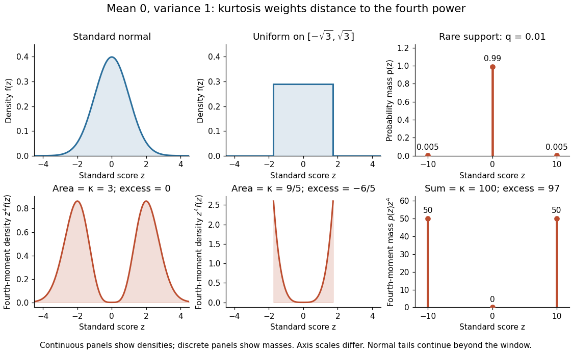
Kurtosis comparison for a standard normal distribution, a continuous uniform distribution, and a rare-outlier three-point distribution
. The upper panels show probability density functions or a probability mass function; the lower panels show their contributions to the fourth central moment. All three probability distributions have mean zero and variance one. Areas in the continuous panels and sums in the discrete panels give kurtosis. The standard normal distribution continues beyond the displayed window; density and mass heights have different meanings. **Details**.

Rare-outlier three-point distribution ( $P (X = 0) = 1 - q, P (X = \pm 1) = q /2$ )

 0  0

For

0 < q \leq 1

, put probability mass

1 - q

at zero and

q /2

at each of

- 1

and

1

. This symmetric probability distribution has mean zero. Its second and fourth moments are both

q

, because the nonzero outcomes have square and fourth power equal to one:

Var (X) = q, E [X^{4}] = q, κ (X) = \frac{q}{q ^{2}} = \frac{1}{q} .

(1)

For

q = 1/4

the kurtosis is

4

; for

q = 1/100

it is

100

. In the latter case

99%

of the probability mass is at zero, yet all of the fourth central moment comes from the remaining

1%

. The standard score

Z = X / q

takes values

0

and

\pm q^{- 1/2}

, with variance one. Each nonzero outcome contributes

\frac{q}{2} (q^{- 1/2})^{4} = \frac{1}{2 q}

(2)

to kurtosis. At

q = 1/100

, the two rare outcomes are ten standard deviations from the mean, and their contributions are

50 + 50 = 100

Figure 1.
Probability mass and fourth-moment contributions for a rare-outlier three-point distribution
. The left panels keep the original support of a probability distribution ${- 1, 0, 1}$ ; the right panels use standard scores. A rare outcome can have small probability mass but a large contribution to kurtosis. Each row is a different specified probability distribution, not a statistical sample. **Details**.

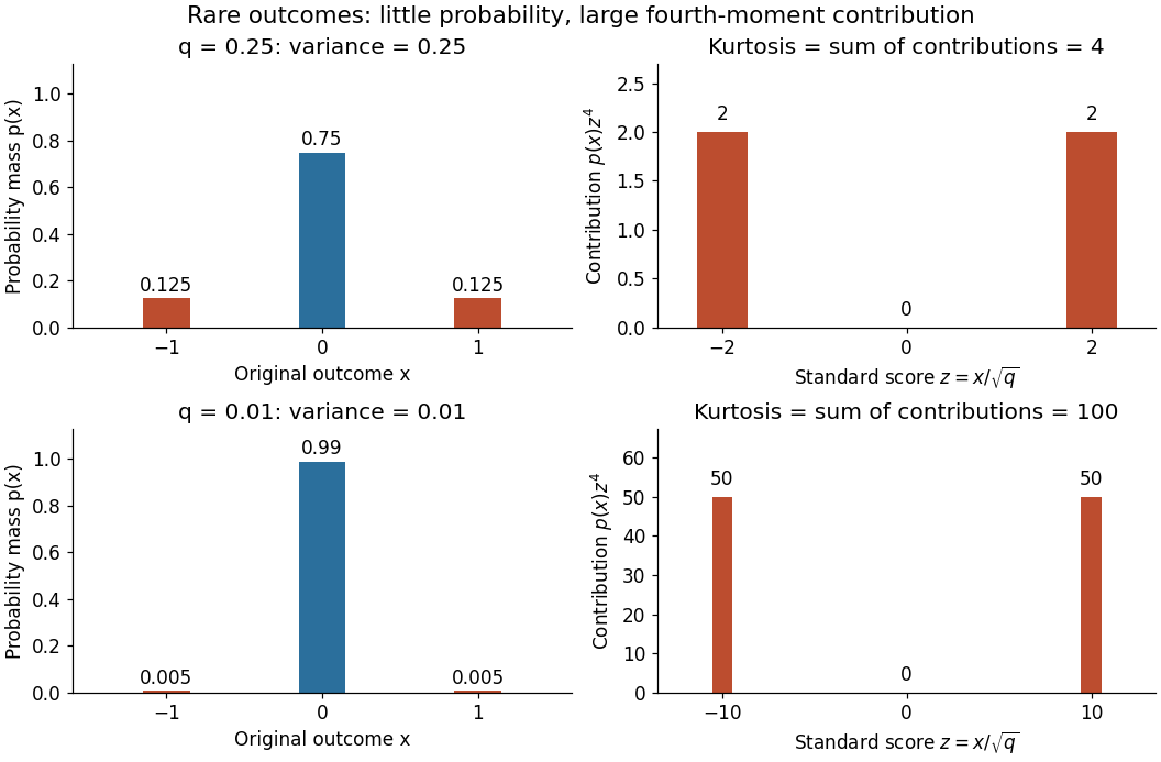
Every member has finite support of a probability distribution, so all its moments are finite. Nevertheless, kurtosis becomes arbitrarily large as

q

approaches zero: high kurtosis does not require an unbounded support of a probability distribution or a heavy-tailed distribution. At

q = 0

the variance vanishes and kurtosis is undefined. At

q = 1/3

this discrete probability distribution even has the normal distribution value

κ = 3

and excess kurtosis zero, so those values do not establish a normal distribution.

Affine invariance of kurtosis ( $κ (a X + b) = κ (X) (a \neq = 0)$ )

 0  0

Changing units or shifting the origin preserves kurtosis. For real constants

a \neq = 0

and

b

, the mean of

Y = a X + b

a μ + b

, its variance is

a^{2} σ^{2}

, and its fourth central moment is

a^{4} E [(X - μ)^{4}]

. The factors

a^{4}

cancel in the ratio, even for negative

a

. Hence excess kurtosis is also unchanged. For example,

100 X + 7

and

X

have the same kurtosis, although their means and variances differ. The case

a = 0

produces zero variance and is excluded.

Central contribution to kurtosis ( $C_{h} = E [Z^{4} 1_{{∣ Z ∣ \leq h}}]$ )

 0  0

For a standard score

Z

and

h > 0

, split kurtosis into the contribution

C_{h}

from within

h

standard deviations of the mean and the contribution

T_{h}

from outside:

κ = C_{h} + T_{h}, C_{h} = E [Z^{4} 1_{{∣ Z ∣ \leq h}}], 0 \leq C_{h} \leq h^{4} .

(1)

The indicator function selects the central outcomes. The bound follows directly from

Z^{4} \leq h^{4}

there. Thus

C_{h} / κ \leq h^{4} / κ

: when kurtosis is large, any fixed central range contributes a small fraction. This is a precise reason to emphasize extreme standard scores rather than peak height.^[ref]

For the rare-outlier three-point distribution with

q = 1/100

C_{1} = 0

and

T_{1} = 100

. At the other endpoint

q = 1

, all probability mass lies at

Z = \pm 1

, so

C_{1} = κ = 1

: central dominance is possible when kurtosis is small. More generally, the Cauchy-Schwarz inequality gives

κ = E [Z^{4}] \geq (E [Z^{2}])^{2} = 1

; the equally weighted outcomes

\pm 1

attain this minimum.

Integrated tail distribution ( $f_{I} (x) = P (X > x) / E X$ )

 0  0

For a positive random variable

X

with finite nonzero expected value

μ

, its integrated tail law has density

f_{I} (x) = P (X > x) / μ

x \geq 0

. The tail integral formula for moments normalizes it. For

r > 0

its exponential transform is

\int e^{r x} f_{I} (x) d x = [M_{X} (r) - 1] / (μ r)

, with extended-value interpretation when needed.

Mixture distribution ( $P = \sum_{j} w_{j} P_{j}$ )

 1  0

A mixture distribution first chooses a component

j

with nonnegative mixture weights

w_{j}

summing to one, then samples from its law

P_{j}

. Consequently

P (A) = \sum_{j} w_{j} P_{j} (A)

, and any finite moment-generating function is the same weighted sum of the component transforms. A component may be a Dirac measure, so a mixture may have both discrete and continuous parts.

Gaussian mixture distribution ( $p (x) = \sum_{j} w_{j} ϕ_{μ_{j}, σ_{j}} (x)$ )

 0  0

A Gaussian mixture distribution is a weighted sum of normal distribution densities, with nonnegative weights summing to one. It need not itself be a normal distribution: components with different means and variances can produce skewness or several modes. Its raw moments are weighted sums of the component moments.

Symmetric rational mixture sampler ( $f_{p} (x) = \frac{p}{π ( 1 + x ^{2} )} + (1 - p) \frac{∣ x ∣}{( 1 + x ^{2} ) ^{2}}$ )

 0  0

The displayed mixture distribution combines a Standard Cauchy distribution and a symmetric law whose magnitude has cumulative distribution function

r^{2} / (1 + r^{2})

for

r \geq 0

. Use independent uniforms

U, V, H

: if

U \leq p

, return

tan (π (V - 1/2))

; otherwise return a fair independent sign times

V / (1 - V)

. The magnitude density is

2 r / (1 + r^{2})^{2}

and splitting its mass equally between signs gives

∣ x ∣/ (1 + x^{2})^{2}

. An alternative rejection sampling proposal is standard Cauchy, with envelope constant

M = p + π (1 - p) /2

, because

∣ x ∣/ (1 + x^{2}) \leq 1/2

Hyperexponential distribution ( $\overline{F} (x) = \sum_{i} w_{i} e^{- r_{i} x}$ )

 0  0

A finite mixture distribution of exponential distributions with rates

r_{i} > 0

and nonnegative weights summing to one. Its expected value is

\sum_{i} w_{i} / r_{i}

and its moment-generating function is

\sum_{i} w_{i} r_{i} / (r_{i} - t)

on the common finite domain. The mixture chooses one component for each observation; it is not a sum of independent exponential variables.

Nonarithmetic distribution

 0  0

A probability distribution is nonarithmetic when it is not concentrated on

d Z

for any

d > 0

. Every law with a probability density is nonarithmetic. This hypothesis removes lattice oscillations from the key renewal theorem.

Right endpoint of a distribution ( $x_{F}$ )

 0  0

The right endpoint of a distribution with distribution function

F

x_{F} = sup {x : F (x) < 1}

, possibly infinite. The survival function is positive below

x_{F}

Joint probability distribution

 0  0

The joint probability distribution of random variables

X_{1}, \dots, X_{n}

is the probability distribution of the random vector

(X_{1}, \dots, X_{n})

. It records both the marginal distributions and their dependence.

Exchangeable random variables

 0  0

A family of random variables is exchangeable if its joint probability distribution is unchanged by finite permutations of its coordinates. Independent and identically distributed random variables are exchangeable, but exchangeable random variables need not be independent random variables.

De Finetti theorem

 0  0

For an infinite sequence of real exchangeable random variables, conditional on its invariant sigma-algebra of an exchangeable sequence, the coordinates are independent and identically distributed. In particular, for Borel sets

A_{0}, \dots, A_{p}

E [\prod_{k = 0}^{p} 1_{A_{k}} (X_{k}) ∣ S] = \prod_{k = 0}^{p} E [1_{A_{k}} (X_{k}) ∣ S] .

(1)

Here is the core proof. Let

S_{m}

denote invariance under permutations of coordinates

0, \dots, m

. Symmetrization as conditional expectation identifies the empirical average of each indicator with its conditional expectation on

S_{m}

. The reverse martingale convergence theorem gives its limit conditional on

S

. Multiplying the averages sums over all ordered coordinate tuples, including repetitions. Symmetrization of the product itself sums over the distinct tuples. The fraction of repeated tuples is at most

(2 p + 1) / (m + 1)

, so these bounded averages have the same limit. This proves the displayed factorization. Permutation invariance also makes the individual conditional laws identical. A regular conditional distribution on the real line packages that common law as a random probability measure, giving the equivalent mixture-of-iid formulation.

Invariant sigma-algebra of an exchangeable sequence ( $S = {A : T_{π}^{- 1} A = A for every finitely supported permutation π}$ )

 0  0

On the coordinate product space of a sequence, the invariant sigma-algebra consists of measurable events unchanged by every finite permutation of coordinates. Its definition is pointwise and does not depend on the probability law. An exchangeable law makes each such permutation measure preserving. Events in the tail sigma-algebra are invariant because any finite permutation fixes every sufficiently late coordinate. Conversely, exchangeable invariant events are tail events modulo null sets.

Exchangeable invariant events are tail events modulo null sets

 0  0

For a real sequence of exchangeable random variables, every event

A

in its invariant sigma-algebra of an exchangeable sequence agrees almost surely with an event of its tail sigma-algebra. Put

F = 1_{A}

. Approximate

F

L^{1}

by its conditional expectation on the first

n + 1

coordinates. Swap that block with the next

n + 1

coordinates. Invariance of

A

and the law shows that the conditional expectation on the second block is an equally good approximation. It is measurable with respect to the tail after index

n

. The L1 contraction of conditional expectation then bounds

∥ F - E [F ∣ G_{n}] ∥_{1}

by twice the approximation error. The reverse martingale convergence theorem gives

F = E [F ∣ ⋂_{n} G_{n}]

almost surely. Thresholding the latter at

1/2

supplies the required tail event. Together with the reverse inclusion, the two sigma-algebras have identical probability completions.

Convolution of independent random variables

 0  0

If independent real random variables

X

and

Y

have densities

f_{X}

and

f_{Y}

, their sum has the convolution density

f_{X + Y} (z) = (f_{X} * f_{Y}) (z) = \int_{- \infty}^{\infty} f_{X} (x) f_{Y} (z - x) d x .

(1)

Gaussian smoothing of an integer-valued distribution ( $g_{σ} (z) = \sum_{n \in Z} p_{n} φ_{σ} (z - n)$ )

 0  0

Let

X

take integer values with probabilities

p_{n}

, and let

Y_{σ}

be an independent centered normal distribution with positive standard deviation

σ

. Conditioning on

X

gives the probability density function of their sum as

g_{σ} (z) = \sum_{n} p_{n} φ_{σ} (z - n)

, where

φ_{σ}

is the normal density. Nonnegativity and Tonelli's theorem show that this density integrates to one. For small

σ

, isolated atoms become narrow smooth peaks with their original probability masses.

For each fixed real

t

, dominated convergence gives

σ g_{σ} (σ t) = E φ_{1} (t - X / σ) ⟶ φ_{1} (t) (σ \to \infty),

(1)

since

X / σ \to 0

almost surely and

φ_{1}

is bounded. Thus every fixed integer-valued distribution acquires a Gaussian central profile on this expanding scale, without any moment assumption on

X

. This is not a claim about uniform relative error in the tails or about finite moments. For example, if

p_{n} = 3/ (π^{2} n^{2})

for

n \neq = 0

and

p_{0} = 0

, the expectation of

∣ X ∣

is infinite. Since

E ∣ Y_{σ} ∣ < \infty

, the triangle inequality forces

E ∣ X + Y_{σ} ∣ = \infty

too. Symmetry then gives equal infinite positive and negative first moments, so there is no ordinary mean. The second moment is also infinite. A Gaussian-looking center can therefore coexist with a heavy-tailed distribution.

Convolution of a Cauchy distribution and a uniform distribution

 0  0

Let

X

have the Standard Cauchy distribution and let

Y

, independently, have the uniform distribution on

[- h, h]

, where

h > 0

. The convolution of probability densities gives the probability density of

Z = X + Y

p_{h} (z) = \frac{1}{2 hπ} \int_{- h}^{h} \frac{d y}{1 + ( z - y ) ^{2}} = \frac{a r c t a n ( z + h ) - a r c t a n ( z - h )}{2 hπ} .

(1)

This is an even function. Its derivative is

p_{h}^{'} (z) = \frac{- 2 z}{π [ 1 + ( z + h ) ^{2} ] [ 1 + ( z - h ) ^{2} ]},

(2)

so its unique mode is zero. Its tails satisfy

p_{h} (z) \sim 1/ (π z^{2})

∣ z ∣ \to \infty

: multiplying the integral by

z^{2}

makes the integrand converge uniformly to

1

on the bounded interval

[- h, h]

. Consequently both positive and negative parts of the first moment diverge, so its expected value does not exist. The symmetric Cauchy principal value of that moment is zero, which is a different assertion. Adding a bounded independent displacement smooths the probability density without removing the divergent first moment of the Cauchy distribution.

Taxi distance convolution on a rectangular road cycle ( $D = A + B$ )

 0  0

For a taxi starting at any vertex of a rectangle with side lengths

s, t

, a uniform pickup vertex gives approach-distance law uniform on

0, s, t, s + t

. Conditional on that pickup, a uniform distinct destination gives passenger-distance law uniform on

s, t, s + t

, independent of the pickup vertex. Hence the two distance variables are independent despite sharing that vertex. Their convolution has twelve equally likely pairs. Its mean is

7 (s + t) /6

and its variance is

(s^{2} + t^{2}) /4 + 2 (s^{2} + t^{2} - s t) /9

. Repeated numerical sums combine their multiplicities when some distances coincide.

Marginal distribution

 0  0

A marginal distribution is the distribution of a selected coordinate or subvector of a random vector, obtained from the joint distribution by integrating or summing over the remaining coordinates.

Marginalization

 0  0

Marginalization sums or integrates a joint probability distribution over unwanted coordinates to obtain a marginal distribution.

Marginal density ( $f_{X} (x) = \int f_{X, Y} (x, y) d y$ )

 0  0

A marginal density is a probability density function for one component of a joint probability distribution. Integrating the joint probability density over the other coordinates gives it; for two components,

f_{X} (x) = \int f_{X, Y} (x, y) d y

Symmetric probability distribution

 0  0

A real probability distribution is symmetric about

m

when

X - m

and

m - X

have the same distribution. A centered normal distribution is symmetric about zero.

Centrally symmetric probability distribution

 0  0

A probability distribution on a vector space is centrally symmetric about zero when

X

and

- X

have the same distribution. Independent observations from such a distribution are jointly invariant under coordinatewise sign changes.

Rademacher distribution

 0  0

A Rademacher random variable takes the values

1

and

- 1

, each with probability

1/2

Rademacher function ( $r_{n} (t) = (- 1)^{⌊ 2^{n} t ⌋}$ )

 0  0

[0, 1)

with Lebesgue measure, the functions

r_{n} (t) = (- 1)^{⌊ 2^{n} t ⌋}

n \geq 1

, are independent symmetric Rademacher random variables. Every prescribed pattern for the first

n

functions occupies a dyadic interval of measure

2^{- n}

. Their closed span in

L^{1}

is isomorphic to the l2 sequence space by the Khintchine inequality.

Rademacher sum ( $S = \sum_{i} a_{i} ϵ_{i}$ )

 0  0

A Rademacher sum is a linear combination of independent Rademacher random variables, with scalar or normed-space-valued coefficients. Its moments are controlled by the Khintchine inequality in the scalar case and the Kahane-Khintchine inequality in a general normed vector space.

Dyadic Rademacher series ( $Y = \sum_{j \geq 1} 2^{- j} X_{j}$ )

 0  0

For independent Rademacher random variables, this series converges absolutely on every sign sequence and has the uniform distribution on

[- 1, 1]

. Its first

n

terms are uniform on the

2^{n}

midpoints of equal subintervals of

[- 1, 1]

, giving weak convergence of probability measures by Riemann sums. The remaining tail has absolute value at most

2^{- n}

, and its mean square is

4^{- n} /3

by independence. Thus convergence is also almost surely and in

L^{2}

Bernoulli function (hypercube, $ϵ_{i} (ω) = ω_{i}$ )

 0  0

On the Boolean hypercube

{- 1, 1}^{d}

with uniform measure, each coordinate is a Rademacher random variable. Products of these sign coordinate functions are Walsh characters. This use of Bernoulli function is distinct from the fluid-mechanical Bernoulli function.

Maximum of finitely many Rademacher linear forms ( $Pr (max_{i} ∣ u_{i}^{T} ξ ∣ \leq α) > 1 - 2 m e^{- α^{2} /2}$ )

 0  0

For independent Rademacher random variables and

∥ u_{i} ∥_{2} \leq 1

, this bound holds for

α > 0

. The moment-generating function satisfies

\prod_{j} cosh (t u_{ij}) \leq e^{t^{2} /2}

, with strict inequality for a nonzero vector and

t > 0

. Applying the exponential Markov bound to both tails and then the union bound proves a strict failure bound; a zero vector has failure probability zero. At

α = 2 lo g (2 m)

, the success probability is strictly positive, ensuring a sign vector with all linear forms below that threshold.

Truncated distribution

 0  0

A truncated distribution is a conditional probability distribution obtained by restricting a random variable to a specified subset of its original support and renormalizing.

Truncated exponential distribution ( $f (u) = \frac{d e ^{- d u}}{1 - e ^{- d t}} 1_{0 < u < t}$ )

 0  0

Condition an exponential distribution of rate

d > 0

on falling below

t > 0

. Normalizing its probability density function gives the displayed density. Integration gives expectation

1/ d - t / (e^{d t} - 1)

. As

d ↓ 0

, the density tends to the uniform distribution on

(0, t)

and the expectation tends to

t /2

// Target: probability-and-statistics.bigb

Upper-endpoint estimation in a truncated distribution ( $M = t_{(n)}$ )

 0  0

For a positive continuous density

f_{θ}

with strictly increasing cumulative distribution function

F_{θ}

, observations from its upper-truncated law have likelihood

\prod_{i} f_{θ} (t_{i}) / F_{θ} (M)^{n}

M > t_{(n)}

. Holding

θ

fixed, decreasing

M

toward

t_{(n)}

increases the likelihood; taking a supremum over

θ

preserves nonincreasing dependence on

M

. Provided the nuisance fit is finite, the usual closed-support endpoint estimate is

t_{(n)}

. With the literal open support

t < M

, only a limiting supremum need exist. A sample maximum is not a validated bound for future observations, and support depending on a parameter prevents automatic application of Wilks theorem.

Zero-truncated claim-count distribution ( $G_{N ∣ N > 0} (z) = \frac{G _{N} ( z ) - G _{N} ( 0 )}{1 - G _{N} ( 0 )}$ )

 0  0

For a nonnegative integer claim count

N

with

p = P (N = 0) < 1

, the conditional law given

N > 0

has masses

P (N = n) / (1 - p)

for

n \geq 1

. Its probability generating function is

(G_{N} (z) - p) / (1 - p)

. Truncation at zero is meaningful only when the positive-count event has positive probability.

Aggregate recursion for zero-truncated Panjer counts ( $g_{k} = p_{1} f_{k} + \sum_{j = 1}^{k - 1} (a + bj / k) f_{j} g_{k - j}$ )

 0  0

Let

N \geq 1

have probability mass function

p_{n}

satisfying

p_{n} = (a + b / n) p_{n - 1}

for

n \geq 2

. Let independent positive integer claim sizes have probability mass function

f_{j}

, independently of

N

. The aggregate probability mass function

g_{k}

satisfies the displayed recursion, with

g_{0} = 0

. To prove it, write

P, F, G

for the count, severity and aggregate probability generating functions. The count recurrence gives

(1 - a z) P^{'} (z) = (a + b) P (z) + p_{1}

. Since

G = P \circ F

, the chain rule gives

(1 - a F) G^{'} = ((a + b) G + p_{1}) F^{'}

. Comparing coefficients of

z^{k - 1}

gives the recursion. The forcing term

p_{1} f_{k}

distinguishes this algorithm from the usual Panjer recursion. For a zero-truncated Poisson distribution with parameter

λ

, take

a = 0

b = λ

and

p_{1} = λ / (e^{λ} - 1)

Truncated normal distribution ( $T N_{A} (μ, σ^{2})$ )

 0  0

A truncated normal distribution is a normal distribution conditioned to lie in a specified subset of the real line. Its density is the original Gaussian density divided by the probability of the retained set.

Gaussian positive-part expectation ( $E [(m + a Z)^{+}] = m Φ (m / a) + a ϕ (m / a)$ )

 0  0

For

Z

with standard normal distribution,

m \in R

, and

a > 0

, integrate

(m + a z) ϕ (z)

over

z > - m / a

. The identity

ϕ^{'} (z) = - z ϕ (z)

gives the displayed expectation of the positive part. This is useful for option pricing when a financial payoff is the positive part of a normal random variable, including a log-call option. At

a = 0

the formula is interpreted by its limit,

m^{+}

Sign-truncated normal sampling

 0  0

To draw

N (μ, 1)

restricted to a positive value, let

a = Φ (- μ)

and return

μ + Φ^{- 1} (a + (1 - a) U)

for uniform

U \in (0, 1)

. For restriction to a negative value use

μ + Φ^{- 1} (a U)

. These are inverse transform sampling constructions. Repeatedly drawing an untruncated normal until its sign agrees is also exact, but inefficient for rare signs.

Beta distribution ( $Beta (α, β)$ )

 1  0

The beta distribution is an absolutely continuous probability distribution for a random variable

X

between zero and one. It can describe uncertainty about a probability, such as an unknown coin's chance of heads. For any real

α, β > 0

, its probability density function is

f_{X} (x) = \frac{x ^{α - 1} ( 1 - x ) ^{β - 1}}{B ( α , β )}, 0 < x < 1,

(1)

and zero outside

[0, 1]

. The normalizer is the Euler beta function, related to the gamma function by the beta-gamma identity:

B (α, β) = \int_{0}^{1} x^{α - 1} (1 - x)^{β - 1} d x = \frac{Γ ( α ) Γ ( β )}{Γ ( α + β )} .

(2)

Thus the probability density function integrates to one. ^[ref].

The endpoint behavior explains why the restrictions are exactly

α, β > 0

: near zero the probability density function behaves like a constant times

x^{α - 1}

, and near one like a constant times

(1 - x)^{β - 1}

. These improper integrals converge for positive parameters, even when the probability density function diverges at zero for

α < 1

or at one for

β < 1

. There is no probability mass at either endpoint:

P (X = 0) = P (X = 1) = 0

. A probability density function's height is not a probability; an interval's probability is the area under it.

Some useful examples of the beta distribution are:

$Beta (1, 1)$ is the uniform distribution on $(0, 1)$ , with probability density function $f_{X} (x) = 1$ .
$Beta (2, 2)$ has probability density function $f_{X} (x) = 6 x (1 - x)$ : values near one half are favored, and it is a symmetric probability distribution about one half.
$Beta (2, 5)$ has probability density function $f_{X} (x) = 30 x (1 - x)^{4}$ . Its mean is $2/7$ and its variance is $10/ (49 \cdot 8) = 5/196 \approx 0.0255102$ ; most of its area lies toward the lower end.
$Beta (1/2, 1/2)$ is the arcsine distribution, with probability density function $f_{X} (x) = 1/ (π x (1 - x))$ . It favors values near both endpoints despite having mean $1/2$ ; its variance is $1/8$ .

Figure 1.
Beta density shapes: uniform, central, asymmetric, and boundary singular
. **Details**.

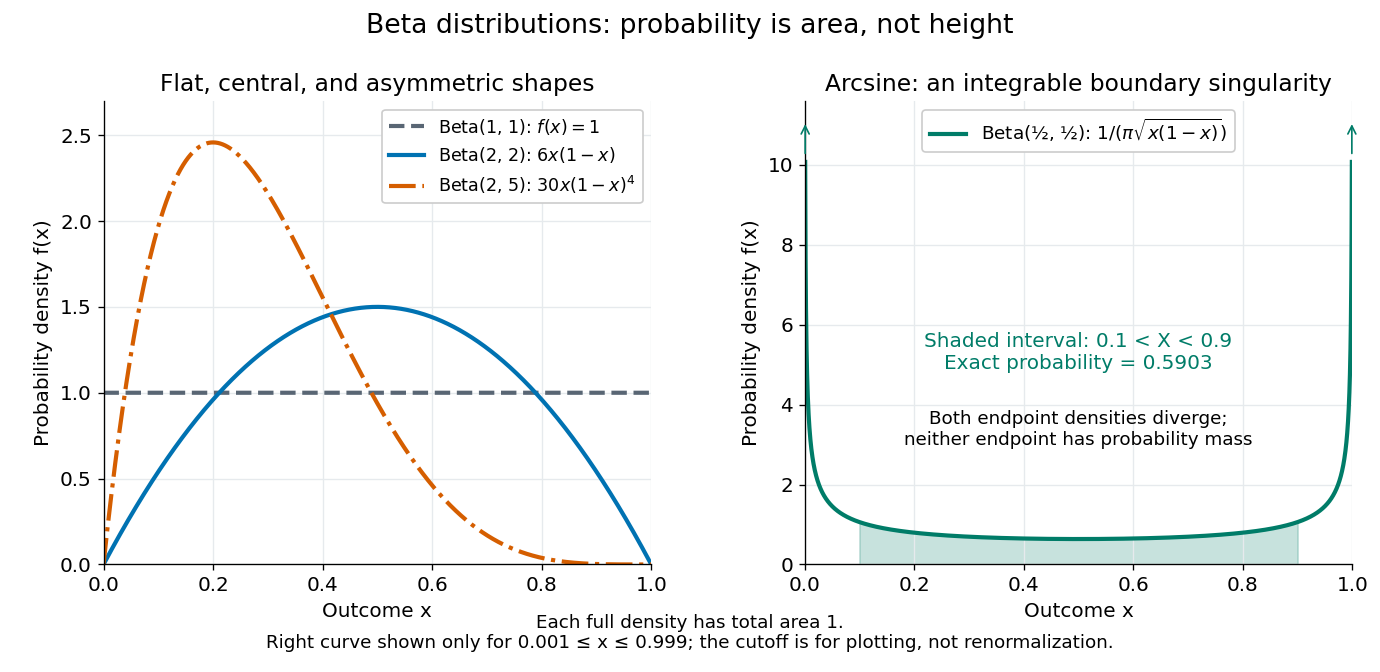
The arcsine distribution curve is plotted only for

0.001 \leq x \leq 0.999

; its finite plotted ends do not represent finite endpoint values of the probability density function. Using the inverse sine, the shaded central interval has exact probability

P (0.1 < X < 0.9) = 1 - 4 arcsin (0.1) / π \approx 0.5903

, calculated analytically rather than by treating the cropped curve as normalized.

To separate location from spread, write

κ = α + β

and

m = α / κ

. The mean and variance of the beta distribution are

E [X] = m = \frac{α}{κ}, Var (X) = \frac{α β}{κ ^{2} ( κ + 1 )} = \frac{m ( 1 - m )}{κ + 1} .

(3)

The mean specifies the balance between the parameters; their sum

κ

controls concentration about that mean. Multiplying both parameters by the same positive number preserves the mean and changes the variance. Larger

κ

puts more area near

m

and makes the probability density function taller there; the total area stays one. Small

κ

allows much greater spread, sometimes favoring the endpoints rather than the mean itself.

For example, keeping mean

m = 0.3

and taking

κ = 5, 20, 80

gives the beta distributions

Beta (1.5, 3.5)

Beta (6, 14)

, and

Beta (24, 56)

. Their variances are

0.035

0.01

, and

0.21/81 \approx 0.00259259

, respectively. Parameters need not be integers.

Figure 2.
The same beta mean with three concentrations and decreasing variance
. **Details**.

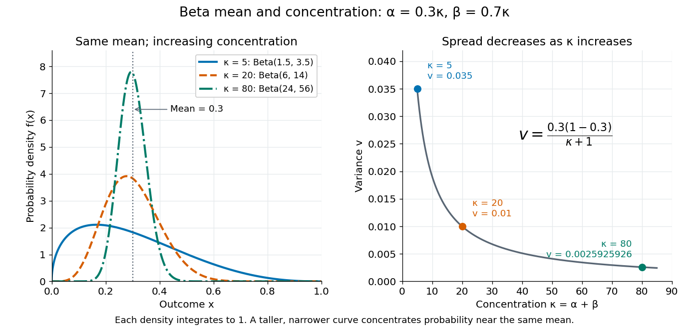
The formulas follow from two short moment calculations. Multiplying the probability density function by

x

x^{2}

increases the first parameter of the Euler beta function:

E [X] = \frac{B ( α + 1 , β )}{B ( α , β )} = \frac{α}{κ}, E [X^{2}] = \frac{B ( α + 2 , β )}{B ( α , β )} = \frac{α ( α + 1 )}{κ ( κ + 1 )} .

(4)

Apply the Gamma function recurrence to the beta-gamma identity, then subtract

(E [X])^{2}

from

E [X^{2}]

to obtain the variance.

The beta distribution is especially convenient as a prior distribution for the unknown success probability

P

of Bernoulli trials. The Beta-binomial conjugacy says that

h

successes and

t

failures update a prior distribution

Beta (α, β)

to a posterior distribution

Beta (α + h, β + t)

. For example, suppose a coin has prior distribution

Beta (2, 2)

and we observe eight heads and two tails. Its posterior distribution is then

Beta (10, 4)

, with posterior mean

5/7

. ^[ref].

Mixed power moments of a beta distribution ( $E [X^{s} (1 - X)^{t}] = B (α + s, β + t) / B (α, β)$ )

 0  0

For

X \sim Beta (α, β)

with positive parameters, and real

s > - α

t > - β

, multiply its density by

x^{s} (1 - x)^{t}

. The resulting integral is a beta function with shifted parameters, hence

E [X^{s} (1 - X)^{t}] = \frac{Γ ( α + β ) Γ ( α + s ) Γ ( β + t )}{Γ ( α ) Γ ( β ) Γ ( α + β + s + t )} .

(1)

The restrictions on the powers are exactly the endpoint-integrability conditions. This includes ordinary moments, reciprocal moments when they exist, and quantities involving both the occupied fraction

X

and remaining fraction

1 - X

. In particular,

s = 1, t = 0

gives

E [X] = α / (α + β)

.^[ref]

Concentration of a beta prior near zero ( $P (Θ > t) = (1 - t)^{β}$ )

 0  0

For

Θ \sim Beta (1, β)

, direct integration of its probability density function gives the displayed tail for

0 < t < 1

. Increasing

β

strictly decreases every such tail probability, and

Θ

converges in probability to zero as

β \to \infty

. Its mean is

1/ (β + 1)

and its variance is

β / [(β + 1)^{2} (β + 2)]

; both decrease for

β > 1

. For the variance, logarithmic differentiation gives

1/ β - 2/ (β + 1) - 1/ (β + 2) < 0

in that range.

After

S

successes in

N

conditionally independent Bernoulli trials, Beta-binomial conjugacy gives posterior mean

(S + 1) / (N + β + 1)

. Its derivative with respect to

β

is negative, while the weight

(β + 1) / (N + β + 1)

assigned to the prior mean is increasing for

N > 0

Estimation of a beta shape parameter ( $θ = - n / \sum_{i} lo g X_{i}$ )

 0  0

For an independent statistical sample from the beta distribution with parameters

(θ, 1)

θ > 0

, the probability density function is

θ x^{θ - 1}

(0, 1)

. Its raw moments are

E X^{r} = θ / (θ + r)

for

r > - θ

, by direct integration. Consequently the method of moments gives

T_{1} = \overset{ˉ}{X} / (1 - \overset{ˉ}{X})

, whereas the maximum-likelihood estimator is

T_{2} = - n / \sum_{i} lo g X_{i}

The second formula follows by setting the score function

n / θ + \sum_{i} lo g X_{i}

to zero; its derivative is negative. Also

- lo g X_{i}

has an exponential distribution of rate

θ

, since

P (- lo g X_{i} > u) = e^{- θ u}

. The central limit theorem and delta method give

n (T_{1} - θ) d N (0, \frac{θ ( θ + 1 ) ^{2}}{θ + 2}), n (T_{2} - θ) d N (0, θ^{2}) .

(1)

Thus the asymptotic relative efficiency of

T_{1}

relative to

T_{2}

1 - (θ + 1)^{- 2}

. The transformed sum has a gamma distribution of shape

n

and rate

θ

, which also gives

E T_{2} = n θ / (n - 1)

for

n > 1

and

Var (T_{2}) = n^{2} θ^{2} / [(n - 1)^{2} (n - 2)]

for

n > 2

Moment matching for a beta prior ( $α = mκ, β = (1 - m) κ$ )

 0  0

Moment matching for a beta prior turns a desired mean and variance for an unknown probability into the parameters of a beta distribution prior. Choose

0 < m < 1

and

0 < v < m (1 - m) .

(1)

Solving the beta distribution mean and variance identities gives

κ = \frac{m ( 1 - m )}{v} - 1, α = mκ, β = (1 - m) κ .

(2)

The strict upper bound on the variance makes

κ > 0

, so both parameters are positive. Substitution gives mean

E [P] = m

and variance

Var (P) = v

exactly. A smaller specified variance at fixed mean produces a more concentrated prior distribution.

For example, a desired prior mean

m = 0.3

and variance

v = 0.01

give

κ = 0.21/0.01 - 1 = 20

, hence the beta distribution prior

Beta (6, 14)

. With the same mean and variance

v = 0.035

, the calculation instead gives

κ = 5

and the broader beta distribution prior

Beta (1.5, 3.5)

. Both appear in the concentration diagram above.

The excluded boundary cases have clear meanings. Zero variance would require

P = m

with certainty, not a beta distribution with finite positive parameters. At the other boundary, any random variable

P \in [0, 1]

satisfies

P^{2} \leq P

, hence variance at most

m (1 - m)

; equality requires

P

to take only the endpoint values zero and one. This is a Bernoulli distribution, not a beta distribution. Thus

v \geq m (1 - m)

cannot be matched by positive finite parameters, and

m = 0

m = 1

is also excluded.

After observing

n = h + t > 0

Bernoulli trials, the Beta-binomial conjugacy makes the posterior mean a weighted average of the prior mean

m

and observed binomial proportion

h / n

E [P ∣ h, t] = \frac{α + h}{κ + n} = \frac{κ}{κ + n} m + \frac{n}{κ + n} \frac{h}{n} .

(3)

This formula gives

κ

a precise interpretation as the prior's weight relative to the sample size in this posterior mean. It does not require fictitious observed counts: the beta distribution parameters can be any positive real numbers. For the eight-head, two-tail example above,

κ = 4

and

m = 1/2

, so the posterior mean is

(4 \cdot 1/2 + 10 \cdot 0.8) /14 = 5/7

// Target: statistical-inference.bigb

Beta sampling by uniform order statistics

 0  0

For positive integers

α, β

, the

α

th order statistic from

α + β - 1

independent uniform distributions on

(0, 1)

has Beta distribution

Beta (α, β)

. Selecting the observations below and above a value

u

gives its probability density function proportional to

u^{α - 1} (1 - u)^{β - 1}

, with normalizing factor

(α + β - 1)! / ((α - 1)! (β - 1)!)

Beta sampling by gamma ratios ( $S / (S + T)$ )

 0  0

Independent gamma distributions

S \sim Γ (α, r)

and

T \sim Γ (β, r)

with a common rate yield a Beta distribution

S / (S + T) \sim Beta (α, β)

. The change of variables

S = w u

T = w (1 - u)

has Jacobian determinant

w

, and factors the joint probability density function into a Beta distribution density in

u

and a gamma distribution density in

w

. In particular, independent chi-squared distributions with

2 α

and

2 β

degrees of freedom give the required ratio.

Cumulative distribution function ( $F_{X} (x)$ )

 1  0

For

a < b

P (a < X \leq b) = F_{X} (b) - F_{X} (a), P (X = x) = F_{X} (x) - F_{X} (x^{-}),

(2)

where

F_{X} (x^{-}) = lim_{t ↑ x} F_{X} (t)

is its left-hand limit. The second formula measures a jump. Thus

P (a \leq X \leq b) = F_{X} (b) - F_{X} (a^{-})

; changing an endpoint is harmless only when its point probability is zero.

For the finite example under probability distribution,

F_{X} (x)

0

below zero,

0.2

[0, 1)

0.7

[1, 3)

, and

1

[3, \infty)

. In particular

F_{X} (1) = 0.7

, but

F_{X} (1^{-}) = 0.2

, so the jump gives

P (X = 1) = 0.5

. For the density example,

F_{Y} (y) = y^{2}

[0, 1]

, and its increase from

1/4

3/4

9/16 - 1/16 = 1/2

When an absolutely continuous probability distribution has probability density function

f

, its cumulative distribution function is

F (x) = \int_{- \infty}^{x} f (t) d t

and

F^{'} = f

almost everywhere. A continuous cumulative distribution function by itself does not guarantee such a density: the Cantor distribution is an important exception.

Integrated cumulative distribution function on a bounded interval ( $\int_{l}^{r} F_{X} (t) d t = r - E [X]$ )

 0  0

If a random variable

X

takes values in

[l, r]

, its cumulative distribution function

F_{X}

satisfies

\int_{l}^{r} F_{X} (t) d t = r - E [X] .

(1)

Indeed

\int_{l}^{r} 1_{{X \leq t}} d t = r - X

for every outcome. Taking expected values and using Tonelli's theorem proves the formula, including when the probability distribution has atoms. For a probability density function

f_{X}

, the same proof reverses the order in

\int_{l}^{r} \int_{l}^{t} f_{X} (x) d x d t = \int_{l}^{r} (r - x) f_{X} (x) d x

. Thus

F_{X} (t) / (r - E [X])

, restricted to

[l, r]

, is a probability density function whenever

E [X] < r

. The reflected construction using

1 - F_{X} (t)

has normalising constant

E [X] - l

and is closely related to an integrated tail distribution.

Singular distribution functions have zero derivative almost everywhere ( $μ ⊥ λ_{1} ⟹ F_{μ}^{'} = 0 λ_{1} -a.e.$ )

 0  0

For

F_{μ} (t) = μ ((- \infty, t])

, every difference quotient at

x

is nonnegative and bounded by

4 μ (B (x, 2∣ h ∣)) / λ_{1} (B (x, 2∣ h ∣))

. The spherical derivative of a singular measure vanishes, so the two-sided derivative is zero Lebesgue almost everywhere. A singular distribution function need not be constant: differentiation almost everywhere does not recover increments without absolute continuity of a function of the function.

Kolmogorov distance ( $d_{K} (F, G) = sup_{z} ∣ F (z) - G (z) ∣$ )

 0  0

The Kolmogorov distance between two probability distributions with cumulative distribution functions

F, G

sup_{z \in R} ∣ F (z) - G (z) ∣

Lattice obstruction to normal approximation

 0  0

If a cumulative distribution function is constant between consecutive lattice points spaced by

h

near zero, then its Kolmogorov distance from the standard normal distribution function is at least half the increase of that function across one such interval. This gives a lower bound of order

h

Probability integral transform ( $F (X) \sim U (0, 1)$ )

 0  0

X

has a continuous cumulative distribution function

F

, then

F (X)

has the uniform distribution on

(0, 1)

. Combined with inverse transform sampling, this constructs the monotone rearrangement

G^{- 1} (F (X))

to a target with quantile function

G^{- 1}

Sequential probability integral transform ( $U_{t} = F_{t} (Y_{t}) ∣ Y_{< t} \sim Unif (0, 1)$ )

 0  0

For correct continuous conditional forecasts, the conditional probability integral transform is uniform given the entire past. Iterating conditional probabilities makes the transformed sequence independent and uniform. Uniformity and serial checks assess absolute predictive calibration using only the forecast distributions and observations.

Uniform convergence of distribution functions to a continuous limit

 0  0

If distribution functions

F_{n}

converge pointwise to a continuous distribution function

F

, then the convergence is uniform. Choose finitely many points whose successive

F

-increments and two tails are small, then use monotonicity to squeeze

F_{n} - F

between its values at adjacent points.

Empirical distribution function ( $F_{n}$ )

 0  0

The empirical distribution function counts the fraction of observations at or below a threshold. For a statistical sample of

n \geq 1

real observations

X_{1}, \dots, X_{n}

, define

F_{n} (x) = \frac{# { i : X _{i} \leq x }}{n} = \frac{1}{n} \sum_{i = 1}^{n} 1_{{X_{i} \leq x}} .

(1)

Each indicator function contributes one exactly when its observation is counted. Equivalently,

F_{n} (x) = P_{n} ((- \infty, x])

, where the empirical measure

P_{n} = n^{- 1} \sum_{i} δ_{X_{i}}

assigns probability mass

1/ n

to each observation, including repeated observations.^[ref]

Choose the illustrative statistical sample

[1, 1, 2, 4, 6]

. Its empirical distribution function is

F_{5} (x) = ⎩ ⎨ ⎧ 0 2/5 3/5 4/5 1 x < 1, 1 \leq x < 2, 2 \leq x < 4, 4 \leq x < 6, 6 \leq x .

(2)

For example,

F_{5} (1) = 2/5

counts both observations equal to

1

F_{5} (3) = 3/5

, and

F_{5} (4) = 4/5

. There is no observation at

3

, so there is no jump there. The five observations produce only four distinct jump locations.

Figure 1.
Building an empirical distribution function by counting observations
. The chosen statistical sample is $[1, 1, 2, 4, 6]$ . Stacked marks retain the two observations at $1$ . Open circles show excluded heights and filled circles show the value at each jump of the right-continuous step function. The right axis gives the cumulative count, five times the empirical distribution function. **Details**.

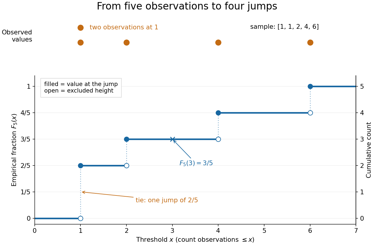
The convention

X_{i} \leq x

makes the empirical distribution function right-continuous: once a threshold reaches an observation, that observation remains counted immediately to its right. For a finite statistical sample, the count is constant from any

x

up to the next larger observed value, proving right continuity. Its left-hand limit

F_{n} (x^{-})

counts observations strictly below

x

, so

F_{n} (x) - F_{n} (x^{-}) = \frac{# { i : X _{i} = x }}{n} .

(3)

A value occurring

m

times causes one jump of size

m / n

. At

1

the jump is

2/5

; at

2

4

, and

6

each jump is

1/5

. All jumps sum to one. Thus the empirical distribution function is a nondecreasing step function with limits zero and one, and is itself a valid cumulative distribution function.

This turns many questions about data into simple cumulative distribution function operations. The observed fraction in

(a, b]

F_{n} (b) - F_{n} (a)

: for

(1, 4]

it is

4/5 - 2/5 = 2/5

, counting

2

and

4

but excluding both

1

s. Including the left endpoint gives

F_{n} (4) - F_{n} (1^{-}) = 4/5

. A sample quantile reads the same staircase in reverse: the smallest threshold reaching

1/2

2

. Unlike a histogram, this representation requires no choice of bins; its jumps retain every observation and its multiplicity.

The exact description of a finite statistical sample must be distinguished from a statistical model for how it was obtained. The empirical distribution function is defined for any finite list, with no independence assumption. Once the list is observed, its counts are fixed. For statistical inference, one often models

X_{1}, \dots, X_{n}

as independent and identically distributed random variables with an unknown population cumulative distribution function

F (x) = P (X_{i} \leq x)

. Then

F

describes the sampling law, while

F_{n}

varies across repeated statistical samples. The value

F_{5} (1) = 0.4

is an observed fraction and an estimate of

F (1)

; it does not establish that the population probability is

0.4

. Even when

F

is continuous, every finite

F_{n}

is discrete.

For any threshold

x

fixed before sampling, the indicator functions are independent Bernoulli random variables with success probability

F (x)

. Therefore the count has a binomial distribution and

n F_{n} (x) \sim Binomial (n, F (x)), E [F_{n} (x)] = F (x), Var (F_{n} (x)) = \frac{F ( x ) ( 1 - F ( x ))}{n} .

(4)

The expected value follows by adding the expected values of the indicator functions; the variance follows by adding their variances using independence and dividing by

n^{2}

. Thus

F_{n} (x)

is an unbiased estimator of

F (x)

at a fixed threshold. Controlling the error at every threshold at once requires more than a fixed-threshold calculation: the DKW inequality supplies such control, and the Glivenko-Cantelli theorem describes its uniform convergence almost surely as

n

grows.

Comparing

F_{n}

with a proposed cumulative distribution function also motivates goodness-of-fit tests, including the Kolmogorov-Smirnov test, the Anderson–Darling test, and the Cramér–von Mises criterion. A standard Kolmogorov-Smirnov test calibration assumes a fully specified continuous population law; fitting its statistical parameters from the same statistical sample changes that calibration.^[ref]

Dvoretzky-Kiefer-Wolfowitz inequality ( $P (sup_{x} ∣ F_{n} (x) - F (x) ∣ > ε) \leq 2 e^{- 2 n ε^{2}}$ )

 1  0

For independent and identically distributed real random variables with cumulative distribution function

F

, the Dvoretzky-Kiefer-Wolfowitz inequality gives, for every

n \geq 1

and

ε > 0

P (sup_{x \in R} ∣ F_{n} (x) - F (x) ∣ > ε) \leq 2 e^{- 2 n ε^{2}} .

(1)

The supremum is the Kolmogorov distance: a single event controls all thresholds simultaneously. The bound holds for discrete, continuous, and mixed probability distributions.^[ref]

For one fixed threshold, Hoeffding's inequality gives the same expression as an upper bound on

P (∣ F_{n} (x) - F (x) ∣ > ε)

. That fixed-threshold result alone does not justify moving the supremum inside the probability. The DKW inequality is the stronger statement needed for a simultaneous empirical distribution confidence band.

Simultaneous empirical distribution confidence band ( $[L_{n} (x), U_{n} (x)]$ )

 0  0

Fix a failure probability

0 < α < 1

and assume an independent and identically distributed statistical sample. A finite-sample confidence band for its population cumulative distribution function is

ε_{n, α} = \frac{l o g ( 2/ α )}{2 n}, L_{n} (x) = max {0, F_{n} (x) - ε_{n, α}}, U_{n} (x) = min {1, F_{n} (x) + ε_{n, α}} .

(1)

Here

lo g

is the natural logarithm. The DKW inequality implies

P (L_{n} (x) \leq F (x) \leq U_{n} (x) for every x \in R) \geq 1 - α .

(2)

This is simultaneous coverage over the whole real line, valid at each fixed sample size.^[ref]

To obtain the band, solve

2 e^{- 2 n ε^{2}} = α

for the positive

ε

. Outside a failure event of probability at most

α

∣ F_{n} (x) - F (x) ∣ \leq ε_{n, α}

for every

x

. Since a cumulative distribution function already lies in

[0, 1]

, clipping the endpoints to this interval preserves the coverage event. The guarantee is at least

1 - α

, and need not equal it.

Choose

α = 0.1

, giving at least

90%

simultaneous coverage under the stated model. For

n = 5, 50, 500

, respectively, the half-widths before clipping are

ε_{5, 0.1} \approx 0.54733, ε_{50, 0.1} \approx 0.17308, ε_{500, 0.1} \approx 0.054733.

(3)

For the chosen five observations, the band at

x = 1

[0, 0.94733]

, while at

x = 4

it is approximately

[0.25267, 1]

. At

x = 3

the unclipped band would be

[0.05267, 1.14733]

, so clipping gives

[0.05267, 1]

. The broad uncertainty is informative: five observations give a precise description of themselves, but a coarse bound for an unknown population cumulative distribution function.

Figure 1.
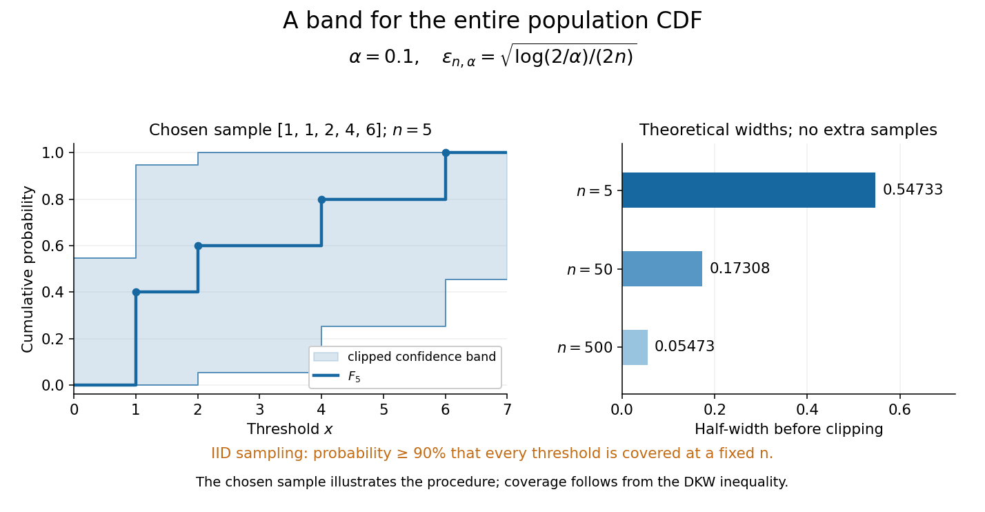
Finite-sample simultaneous uncertainty around an empirical distribution function
. Left: the chosen five observations give $F_{5}$ and its band clipped to $[0, 1]$ , using $α = 0.1$ . Right: theoretical half-widths for $n = 5, 50, 500$ , with no additional samples constructed. The confidence band has coverage at least $90%$ under independent and identically distributed sampling; the drawing illustrates the procedure and does not establish its coverage. **Details**.

A collection of

90%

pointwise confidence intervals only promises coverage separately at each preselected threshold; it does not promise

90%

coverage of an entire cumulative distribution function. Here the one simultaneous event permits inspecting any threshold after seeing the data. The probability refers to repeated sampling of the entire statistical sample, with

F

fixed. It does not assign

90%

probability to a fixed

F

after observing this particular band, and it is not a prediction interval for a future observation. The displayed

n = 5, 50, 500

comparison gives a guarantee for each fixed

n

separately, not simultaneous validity over all sample sizes or an optional stopping rule. The chosen observations are an illustration; the coverage claim follows from the DKW inequality, not from their appearance or a simulation. Dependence or observations with different sampling laws require another argument.

At fixed

α

, multiplying

n

100

divides the half-width by

10

. Conversely, a desired half-width

δ > 0

is ensured by

n \geq lo g (2/ α) / (2 δ^{2})

, rounded up to an integer. For

α = 0.1

and

δ = 0.1

, this sufficient sample size is

150

. This makes the confidence band useful for planning how many observations are needed before estimating threshold probabilities to a chosen simultaneous accuracy.

Anderson–Darling test ( $n \int \frac{( F _{n} - F _{0} ) ^{2}}{F _{0} ( 1 - F _{0} )} d F_{0}$ )

 0  0

The test rejects for large values of this tail-weighted empirical discrepancy. For a specified continuous null, its standard limiting statistic is

\int_{0}^{1} B^{0} (u)^{2} / [u (1 - u)] d u

, using a Brownian bridge. The reciprocal variance weight gives tail deviations more influence than the Cramér–von Mises criterion. If null parameters are estimated, fitting must be included when computing or simulating its reference law.

Cramér–von Mises criterion ( $n \int (F_{n} - F_{0})^{2} d F_{0}$ )

 0  0

This goodness-of-fit criterion integrates the squared difference between the empirical distribution function and a specified continuous null distribution. Under a fully specified null, the probability integral transform makes its law distribution-free; its limiting law is

\int_{0}^{1} B^{0} (u)^{2} d u

for a Brownian bridge. Parameter fitting changes that calibration.

Empirical distribution process ( $α_{n} (x) = n (G_{n} (x) - G (x))$ )

 0  0

The empirical distribution process is the centred, scaled empirical distribution function of an independent sample with cumulative distribution function

G

. Its mean is zero and its covariance is

G (min (x, y)) - G (x) G (y)

. This follows by expanding the two indicator averages: different sample indices have zero covariance, while the same index contributes the covariance of the two nested events. The scaling by

n

keeps these covariances independent of

n

Donsker theorem for empirical distribution functions ( $n (F_{n} - F) ⇝ G_{F}$ )

 0  0

For an independent sample with cumulative distribution function

F

, the empirical distribution process converges in the supremum norm on

ℓ^{\infty} (R)

to the F-Brownian bridge. The convergence uses outer expectation and inner expectation when finite-sample Borel measurability fails. It is a full function-space theorem, stronger than the Finite-dimensional Brownian bridge limit of an empirical distribution process. No continuity of

F

is required. The continuous mapping theorem gives convergence of the supremum statistic; for continuous

F

, its range contains

(0, 1)

and the bridge vanishes at zero and one, giving the Kolmogorov-Smirnov theorem. The function-space statement is stated here as a theorem; its tightness assertion is an additional ingredient beyond the finite-dimensional covariance calculation.

Finite-dimensional Brownian bridge limit of an empirical distribution process

 0  0

For fixed

x_{1}, \dots, x_{d}

, the vector

(α_{n} (x_{j}))_{j = 1}^{d}

converges in distribution to

(B (G (x_{j})))_{j = 1}^{d}

, where

B

is a standard Brownian bridge. To prove it, write the vector as

n^{- 1/2}

times the sum of independent centred bounded indicator vectors. Their covariance matrix is

G (min (x_{i}, x_{j})) - G (x_{i}) G (x_{j})

. The multivariate central limit theorem gives a centred multivariate normal distribution with this covariance, exactly the bridge vector. Singular covariance matrices, including endpoint times or repeated values of

G

, cause no problem. This is a finite-dimensional assertion; a full function-space limit additionally requires tightness.

Cauchy distribution ( $Cauchy (x_{0}, γ)$ )

 0  0

The Cauchy distribution with location

x_{0}

and scale

γ > 0

has probability density function

f (x) = \frac{1}{πγ ( 1 + (( x - x _{0} ) / γ ) ^{2} )} .

(1)

The standard Cauchy distribution has

x_{0} = 0

γ = 1

, characteristic function

e^{- ∣ t ∣}

, and infinite first absolute moment.

Cauchy convolution semigroup ( $K_{a} * K_{b} = K_{a + b}, K_{a} (x) = a / [π (x^{2} + a^{2})]$ )

 0  0

The normalized Cauchy distribution densities

K_{a}

a > 0

, form a convolution semigroup: convolution adds their scale parameters. This follows from the convolution theorem, since their Fourier transforms are proportional to

e^{- a ∣ k ∣}

. Consequently an integral equation with a Cauchy kernel can be solved by subtracting scale parameters when the resulting scale is positive.

Tangent of a uniform angle has a Cauchy distribution ( $s tan Θ \sim Cauchy (0, s)$ )

 0  0

s > 0

and

Θ

has the continuous uniform distribution on

(- π /2, π /2)

, then

Y = s tan Θ

has the Cauchy distribution with location zero and scale

s

. The tangent function is strictly increasing on this interval, so its cumulative distribution function is

P (Y \leq y) = \frac{1}{2} + \frac{1}{π} arctan \frac{y}{s} .

(1)

Differentiating gives the probability density function

s / [π (s^{2} + y^{2})]

. The probability of either endpoint is zero, so including endpoints in the uniform interval does not alter this probability distribution. The slow quadratic decay makes the expected value undefined: its positive and negative parts both have infinite integrals. Its second moment is also infinite, so it has no finite standard deviation.

Cauchy sample mean has an unchanged distribution ( $(X_{1} + \dots + X_{n}) / n \sim Cauchy (0, 1)$ )

 0  0

Independent standard Cauchy distribution variables sum to a Cauchy law of scale

n

, so their sample mean has its original distribution for every sample size. This follows by induction using convolution of probability densities. It does not contradict the usual weak law of large numbers, since the Cauchy law has no finite first absolute moment and its expectation is undefined. Symmetry does not turn a divergent expectation into zero.

Half-Cauchy distribution ( $f (x) = 2 γ / [π (γ^{2} + x^{2})], x > 0$ )

 0  0

The absolute value of a centered Cauchy distribution variable with scale

γ > 0

has this probability density function. Its positive support and doubled density distinguish it from the two-sided distribution. Its unit-scale case arises as the ratio of two independent, equally scaled half-normal distribution variables.

Standard Cauchy distribution

 0  0

The standard Cauchy distribution is

Cauchy (0, 1)

, with density

1/ [π (1 + x^{2})]

and characteristic function

e^{- ∣ t ∣}

Cauchy law of an infinite-horizon Brownian exponential integral ( $\int_{0}^{\infty} e^{W_{s} - s /2} d B_{s} \sim Cauchy (0, 1)$ )

 0  0

For independent Brownian motions

W, B

, the strong law for Brownian motion makes

\int_{0}^{\infty} e^{2 W_{s} - s} d s

finite almost surely, so bracket localization gives an almost sure limit of the stochastic integral. The arctangent transform of a two-noise affine diffusion and endpoint convergence of a bounded angle diffusion identify its distribution function as

1/2 + arctan (x) / π

. Conditional Gaussianity rules out atoms.

Characteristic function of the Cauchy distribution

 0  0

For

X \sim Cauchy (x_{0}, γ)

E [e^{i tX}] = e^{i x_{0} t - γ ∣ t ∣} .

(1)

In particular, the Standard Cauchy distribution has characteristic function

e^{- ∣ t ∣}

Cauchy random variable

 0  0

A Cauchy random variable is a random variable having a Cauchy distribution. For a standard Cauchy random variable

V

E e^{i t V} = e^{- ∣ t ∣} .

(1)

Stability of the Cauchy distribution

 0  0

X_{1}, \dots, X_{n}

are independent standard Cauchy random variables, then

\frac{X _{1} + \dots + X _{n}}{n}

(1)

is again standard Cauchy. Indeed, its characteristic function is

(e^{- ∣ t ∣/ n})^{n} = e^{- ∣ t ∣}

Stable distribution

 0  0

A probability distribution is stable when every linear combination of independent copies has the same distribution up to a location and scale change. The Cauchy distribution is stable with stability parameter one.

Symmetric stable distribution ( $ϕ (t) = exp (i μ t - c ∣ t ∣^{α}), 0 < α \leq 2$ )

 0  0

A symmetric stable distribution has this characteristic function, with

c > 0

and location

μ

. At location zero it is a strictly stable distribution: weighted sums of independent copies have scale factor

(\sum_{j} ∣ a_{j} ∣^{α})^{1/ α}

. The index

α

need not permit a finite mean or variance. The scale in this convention is

c^{1/ α}

, so the coefficient of

∣ t ∣^{α}

and the scale parameter should not be confused.

Cosine integral for a symmetric stable exponent ( $\int_{0}^{\infty} (1 - cos u) u^{- 1 - α} d u = π / [2Γ (1 + α) sin (π α /2)]$ )

 0  0

For

0 < α < 2

, represent

u^{- 1 - α}

Γ (1 + α)^{- 1} \int_{0}^{\infty} v^{α} e^{- vu} d v

. The Tonelli theorem applies to the nonnegative integrand. The inner integral in

u

1/ [v (1 + v^{2})]

, leaving

Γ (1 + α)^{- 1} \int_{0}^{\infty} v^{α - 1} / (1 + v^{2}) d v

. Substitution

z = v^{2}

and the Euler beta function together with the Gamma reflection formula give the result. The bounds at zero and infinity explain exactly the index range.