Solution
ID: past-exam-of-the-mathematics-course-of-the-year-1-of-the-natural-sciences-course-of-the-university-of-cambridge/2002/paper-2/12/b/solution
Past exam of the mathematics course of the year 1 of the natural sciences course of the University of Cambridge 2002 Paper 2 12 b Solution by  Codex 0 2026-10-20
Set both first partial derivatives equal to zero:Thus and , independently, giving exactly nine stationary points. The Hessian matrix is diagonal everywhere:Its diagonal entries are its eigenvalues, so the second-derivative test immediately classifies the points:
- At , the Hessian matrix has eigenvalues . These two points are strict local maxima, each with .
- At , the Hessian matrix has eigenvalues . These two points are strict local minima, each with .
- At , the Hessian matrix has eigenvalues , so it is a saddle point of a scalar function with .
- At , with all four sign combinations, the Hessian matrix has eigenvalues . These four points are saddle points of a scalar function, each with .
In particular,All nine stationary points are nondegenerate, so no higher-order test is needed. Neither type of local extremum is global: as , whereas as .
To organize the contour plot, complete the squares:The level set through all four outer saddle points of a scalar function factors exactly:It is therefore the union of the circle and the hyperbola , which cross at those four saddle points of a scalar function. Near the origin, , so the zero contours have tangents . These two exact structural features, together with the nested contours around the four local extrema, determine the requested sketch. They are an example of a separable quartic landscape with nine stationary points.
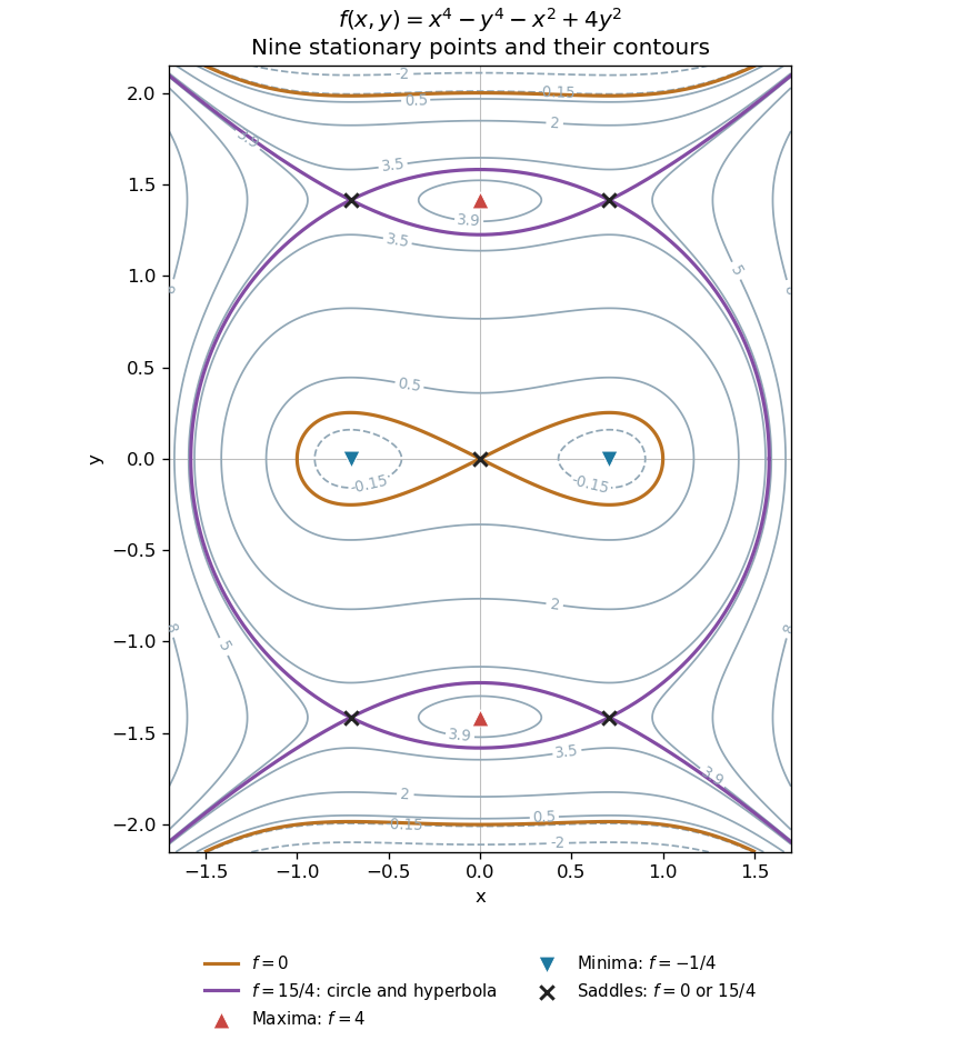
All nine stationary points and contours of the separable quartic
. Original contour plot of . The two maxima, two minima and five saddles are marked. The exact level is highlighted as a circle and a hyperbola intersecting at the four outer saddles; the zero contour crosses at the origin. Details.
New to topics? Read the docs here!