A scalar λ is an eigenvalue of a linear operator A:V→V whenfor some nonzero vector v, called an eigenvector. The scalar must belong to the field over which V is a vector space. Geometrically, a real eigenvalue tells us what A does along a special line: every vector on that line is multiplied by the same number. The eigenvector gives the line and the eigenvalue gives its scaling.
Av=λv
For a real eigenvalue, λ>0 preserves the orientation along the line, λ<0 reverses it, and λ=0 collapses the line to zero. The length is multiplied by the modulus ∣λ∣, so ∣λ∣>1 stretches and 0<∣λ∣<1 contracts. For example, the diagonal matrix diag(2,−1/2,0) doubles one coordinate direction, reverses and halves another, and annihilates the third. Its eigenvalues are 2,−1/2,0; the last direction lies in its kernel.
For a finite square matrix, the eigenvalues are the roots of a polynomial pA, its characteristic polynomial:Here I is the identity matrix. The reason is that Av=λv means (A−λI)v=0 with v=0: the shifted matrix must have a nontrivial kernel, equivalently a zero determinant. The worked symmetric matrix example in eigenvector shows both stages: find the eigenvalues, then find their eigenspaces.
pA(λ)=det(λI−A)=0.
Eigenvalues are especially useful for repeated application of a linear map. If Av=λv, thenOne multiplication proves the next step, so a matrix power becomes an ordinary power on each eigenvector. This explains growth, decay, and alternating signs along these directions. Gilbert Strang develops this connection, and its extension to the matrix exponential, in his lecture "Eigenvalues and Eigenvectors" (MIT 18.065, 2018).[ref]
Anv=λnv(n≥0).
A documented historical connection is C. G. J. Jacobi's "Über ein leichtes Verfahren die in der Theorie der Säcularstörungen vorkommenden Gleichungen numerisch aufzulösen" (1846, Journal für die reine und angewandte Mathematik 30, pp. 51–94). Its opening discusses symmetric matrices arising from small oscillations, with a common unknown subtracted from every diagonal entry. In modern notation this is (A−λI)v=0; Jacobi seeks the parameter and the ratios of the components of v. This is evidence of an early physical and computational setting for the eigenvalue problem, without assigning its discovery to a single person.[ref]
https://doi.org/10.1515/crll.1846.30.51. Jacobi's 1846 paper: original publication
[ref]https://geographiclib.sourceforge.io/geodesic-papers/jacobi-V7.pdf. Jacobi's collected works, volume VII, opening section of the 1846 paper
An eigenvalue collision occurs when distinct branches of eigenvalues coincide in a parameter-dependent family of matrices or linear operators. The resulting repeated eigenvalue need not retain a full eigenbasis; its geometric and algebraic multiplicities must be compared to decide diagonalizability.
The spectral abscissa is the largest real part of a matrix's eigenvalues. It describes asymptotic exponential rates of its matrix exponential, but a non-normal matrix can also have transient amplification. It is generally distinct from the Euclidean logarithmic norm, which gives an immediate Euclidean energy-growth bound.
Geometric multiplicity is the dimension of an eigenspace; algebraic multiplicity is its multiplicity as a root of the characteristic polynomial. For a real symmetric matrix they coincide because it has an orthonormal eigenbasis.
Zero is an eigenvalue of a linear operator exactly when the operator has a nontrivial kernel. Its eigenvectors are precisely the nonzero vectors in that kernel.
ConsiderIts row sums vanish, so (1,1,1)T is an eigenvector for the zero eigenvalue. Its characteristic polynomial iswith sum of principal minors of order twoThe other eigenvalues are (−S±S2−4T)/2. No symmetry is required for this formula; positive diagonal symmetrization of a matrix is a sufficient condition for real roots.
B=−(a+b)cea−(c+d)fbd−(e+f).
det(λI−B)=λ(λ2+Sλ+T),S=a+b+c+d+e+f,
T=ad+bc+bd+ae+af+bf+ce+cf+de.
An eigenvalue problem asks for the eigenvalues and corresponding eigenvectors or eigenfunctions of a linear operator. It is commonly written as the eigenvalue equation Av=λv.
An eigenfunction is a nonzero function f satisfying Lf=λf for a linear operator L and scalar eigenvalue λ.
A nodeless real eigenfunction has no zero in the interior of the domain. For a one-dimensional confining Schrödinger operator, the nodeless theorem for a one-dimensional ground state identifies the ground state as the eigenfunction that can be chosen strictly positive. Normalizable excited states have nodes.
A Dirichlet eigenfunction is an eigenfunction of a differential operator satisfying a homogeneous Dirichlet boundary condition. The term applies to more general boundary-value operators as well as the Dirichlet Laplacian.
An adjoint eigenfunction is a nonzero eigenfunction of the adjoint operator on its adjoint domain. For an inner product conjugate-linear in its first argument, L∗g=λg implies ⟨g,(L−λ)f⟩=0 for every f in the domain of L. Consequently a necessary solvability condition for (L−λ)f=h is ⟨g,h⟩=0. If L−λI is a Fredholm operator, orthogonality to every element of its adjoint kernel is also sufficient. Boundary conditions and weights in a coupled system enter the adjoint domain and must be derived by integration by parts; copying the original eigenfunction without checking them can give a wrong projection.
A generalized eigenfunction solves the eigenvalue equation for a linear operator in an enlarged space, often a space of distributions, although it may fail to belong to the underlying Hilbert space. A plane wave eikx on the whole real line is a generalized momentum eigenstate, with momentum ℏk, and is not square-integrable. This usage differs from a generalized eigenvector in a Jordan chain, where a higher power of L−λ vanishes rather than L−λ itself.
A nonzero vector v is an eigenvector of a linear operator A when Av=λv for some eigenvalue λ. For a real vector space and λ=0, the line through v is preserved: the image can point forward or backward, but cannot turn away from that line. When λ=0, the image is zero and has no direction. The zero vector is excluded because it satisfies the equation for every scalar and identifies no special direction.
Every nonzero scalar multiple of an eigenvector is an eigenvector for the same eigenvalue, since A(cv)=cAv=λ(cv). Thus there is usually no preferred length or sign; choosing a unit vector is a convenient normalization. Eigenvectors for a fixed eigenvalue, together with zero, form its eigenspace.
For a fully computed example, consider the real symmetric matrixIts characteristic polynomial isFor λ=3, (A−3I)v=0 gives −x+y=0, so v3=(1,1)T is an eigenvector. For λ=1, (A−I)v=0 gives x+y=0, so v1=(1,−1)T is an eigenvector. Direct multiplication checks both:The map stretches the line y=x threefold and fixes the line y=−x pointwise. These eigenvectors are orthogonal because v3Tv1=0; dividing each by 2 gives an orthonormal basis. A general vector turns because its components along these two lines receive different scalings. For example, (1,0)T maps to (2,1)T and is not an eigenvector.
A=(2112),A(xy)=(2x+yx+2y).
pA(λ)=det(λ−2−1−1λ−2)=(λ−2)2−1=(λ−3)(λ−1).
Av3=(33)=3v3,Av1=(1−1)=v1.
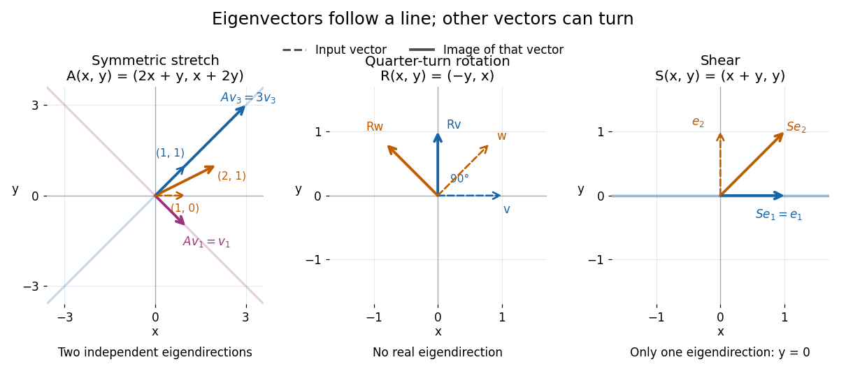
A contrasting example is the planar rotation through 90 degrees:Every nonzero real vector turns to a perpendicular direction, so there are no real eigenvectors. Its characteristic polynomial is λ2+1, which has no real roots. Over the complex numbers, however, R(1,−i)T=i(1,−i)T and R(1,i)T=−i(1,i)T. The same matrix therefore has an eigenbasis in C2 even though it has none in R2: the choice of field matters.
R=(01−10),R(xy)=(−yx).
A zero mode is a nonzero eigenvector of an operator with eigenvalue zero. For a differential fluctuation operator it must also satisfy the specified boundary conditions. A zero mode prevents ordinary inversion of the operator and makes its unmodified functional determinant vanish. Gauge directions can produce zero modes of a kinetic operator, while stationary-path focusing can produce them in a semiclassical boundary-value problem. Removing, separately integrating or otherwise treating these directions is necessary before using a Gaussian determinant formula.
Applying the product of the other eigenvalue factors to a linear relation isolates each coefficient. Distinct eigenvalues therefore give linearly independent eigenvectors. A complete eigenvector basis diagonalizes the associated linear system of ordinary differential equations.
For an eigenvalue λ of a linear operator A:V→V, its eigenspace isIt contains all eigenvectors for λ and the zero vector. Including zero makes this a linear subspace: if v,w∈Eλ, then A(av+bw)=λ(av+bw) for any scalars a,b. Every nonzero vector in this linear subspace has the same scaling under A. Its dimension is the geometric multiplicity of the eigenvalue. If λ is not an eigenvalue, the shifted kernel is only {0}.
Eλ=ker(A−λI)={v∈V:Av=λv}.
For the symmetric matrix A=(2112) from eigenvector,Each eigenspace is a line. An eigenspace can also be a plane or the whole vector space: for B=diag(2,2,5), E2={(x,y,0)T:x,y∈R} is a plane of dimension two, while for C=2I every vector belongs to E2. A repeated eigenvalue therefore need not prevent diagonalizability.
E3=span{(1,1)T},E1=span{(1,−1)T}.
The useful unit of information is the whole eigenspace, rather than a particular choice of eigenvectors inside it. On Eλ, A is simply multiplication by λ. Distinct eigenspaces fit together as a direct sum, and a finite-dimensional linear operator is diagonalizable exactly when they fill the whole vector space. For the example above, every vector splits uniquely asThis decomposition makes the independent scalings visible without multiplying out the original matrix again.
(xy)=2x+y(11)+2x−y(1−1).
An eigenline is a one-dimensional vector subspace spanned by an eigenvector. If Av=λv with v=0, then A(av)=λav for every scalar a, so the line is an invariant subspace. It can be contained in an eigenspace of larger dimension; an eigenline need not be the whole eigenspace.
If a real linear operator A on an n-dimensional vector space has n distinct real eigenvalues, any real square root B commutes with A and preserves each one-dimensional eigenspace. There B is multiplication by a real bi, hence λi=bi2≥0. Conversely, if all the eigenvalues are nonnegative, choosing bi=λi on an eigenbasis supplies a real square root. Without simple spectrum the necessity fails: a real quarter-turn squares to −I.
The vector space of functions satisfying Δf=λf for a specified Laplace-Beltrami operator. On a closed manifold its dimension is finite and is the spectral multiplicity of λ. A finite isometric group action preserves this space; invariant elements are the Laplacian eigenfunctions on the corresponding smooth quotient.
An eigenvalue is simple when it has algebraic multiplicity one.
For unit left eigenvector u and right eigenvector v of a real matrix at a simple eigenvalue λ, its normwise sensitivity isIt measures the first-order amplification of a matrix perturbation into an eigenvalue perturbation.
s(λ)=∣uTv∣1.
If A(t)=A+tE and λ(t) is a differentiable function defining a simple eigenvalue, thenThe Cauchy-Schwarz inequality and the operator norm give
λ′(0)=uTvuTEv.
∣λ′(0)∣≤∥E∥2s(λ).
A finite-dimensional linear operator is diagonalizable over a specified field when it has an eigenbasis. Equivalently, its matrix A admitswhere P is an invertible matrix whose columns are eigenvectors, and D is a diagonal matrix of the corresponding eigenvalues. This change of basis reveals a linear map as independent one-dimensional scalings. The matrix may look coupled in the original coordinates, but each coordinate in the eigenbasis evolves on its own.
A=PDP−1,D=diag(λ1,…,λn),
For the symmetric matrix A=(2112) computed in eigenvector, takeThen AP=PD, hence P−1AP=D. The orthonormal basis version is Q=P/2, an orthogonal matrix satisfying QTAQ=D. Every real symmetric matrix has an orthonormal eigenbasis by the spectral theorem; a general diagonalizable matrix need not have orthogonal eigenvectors.
P=(111−1),P−1=21(111−1),D=(3001).
The immediate payoff is repeated application: adjacent factors P−1P cancel, giving An=PDnP−1. In this example,The component in E3 grows while the component in E1 stays fixed. After division by its Euclidean norm, this particular sequence approaches (1,1)T/2. This is the mechanism behind the power method; an initial vector entirely in E1 would stay there and never find the dominant eigenvalue 3.
An=21(3n+13n−13n−13n+1),An(10)=21(3n(11)+(1−1)).
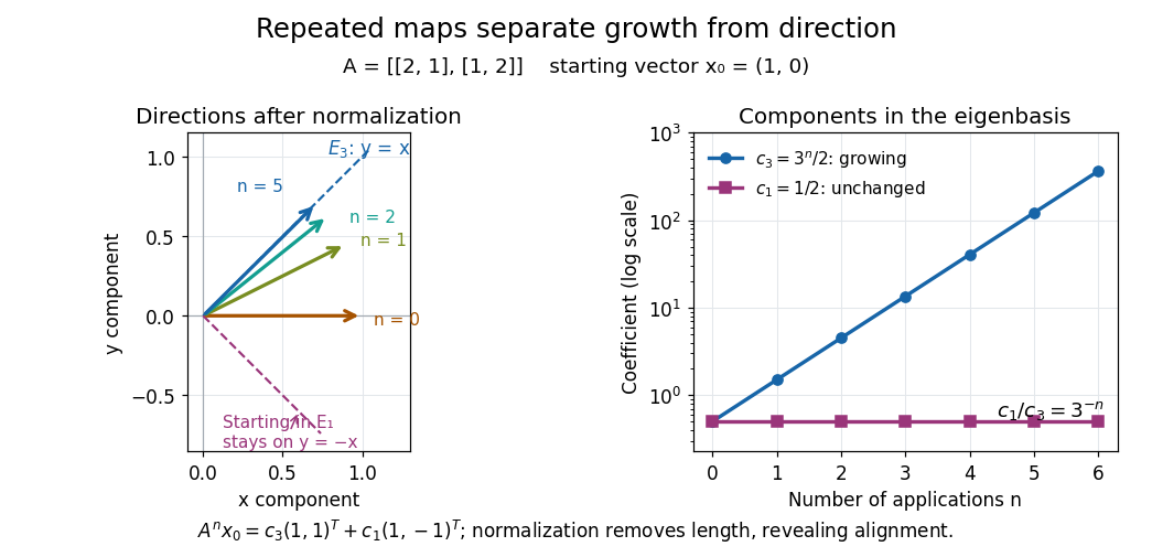
Repeated maps: eigenvalue growth, alignment, and the exceptional starting direction
. Details. Two different obstructions deserve comparison. The planar rotation R in eigenvector is diagonalizable over C but not over R, because its eigenvalues are i and −i. By contrast, the shear mappinghas only λ=1, of algebraic multiplicity two, and E1=span{(1,0)T}, of geometric multiplicity one. There is no second independent eigenvector, even over C. This is a defective matrix, already a two-dimensional Jordan block. Its powers areThus even though both eigenvalues are one, repeated application can produce growth. Eigenvalues alone miss the coupling recorded by a Jordan block. A repeated eigenvalue is harmless when it has enough independent eigenvectors, as I demonstrates. More generally, a matrix is diagonalizable exactly when its characteristic polynomial splits over the chosen field and every eigenvalue has equal geometric multiplicity and algebraic multiplicity. The proof outline is to join bases of the distinct eigenspaces; their direct sum fills the space exactly under these conditions.
S=(1011),(S−I)(xy)=(y0)
Sn=(10n1),Sn(01)=(n1).
A physical motivation is the separation of normal modes. Consider two equal masses m between three identical springs of stiffness k, with the outer ends fixed. By Hooke's law and Newton's second law, the displacement vector q=(q1,q2)T obeysThe eigenvectors (1,1)T and (1,−1)T have eigenvalues 1 and 3: the masses move together in the first normal mode and oppositely in the second. Writing q=a(t)(1,1)T+b(t)(1,−1)T separates the coupled equations into two harmonic oscillators,Their angular frequencies are k/m and 3k/m; the eigenvalues give squared angular frequencies after multiplication by k/m. This is the beauty of diagonalization: finding the right directions turns interacting motions into independent patterns. For a physical treatment, see Yen-Jie Lee's "Coupled Oscillators, Normal Modes" (MIT 8.03SC, 2016), and the local article normal modes of two equal masses between three springs.[ref]
mq¨=−kKq,K=(2−1−12).
a¨+mka=0,b¨+m3kb=0.
A diagonalization is a factorization A=PDP−1 in which D is diagonal and the columns of P form an eigenvector basis.
Let A be invertible over an algebraically closed field. If Am is diagonalizable for some m>0, then A is diagonalizable. Indeed, a nontrivial Jordan block A∣E=λI+N has λ=0 andThe first nonzero nilpotent term prevents this power from being diagonalizable.
(λI+N)m=λmI+mλm−1N+⋯.
Suppose real matrices A,B satisfy AP=PB for an invertible complex matrix P=X+iY. Then AX=XB and AY=YB. The real polynomial det(X+tY) is not identically zero because its value at t=i is nonzero, so some real t makes X+tY invertible. This real matrix intertwines A and B.
Eigenvectors belonging to distinct eigenvalues are linearly independent. Consequently, an n-dimensional operator with n distinct eigenvalues is diagonalizable.
A spectral decomposition expresses a linear operator through its eigenvalues and projections onto its eigenspaces.
An eigenvalue is dominant when its modulus is greater than or equal to that of every other eigenvalue. It is uniquely dominant when the inequality is strict.
A spectral gap is a positive separation between designated parts of the spectrum of a linear operator. For the power method, the relevant gap separates the modulus of the dominant eigenvalue from the other eigenvalue moduli.
Suppose H≥0 has ground energy zero and positive spectral gap at least g, and 0≤V≤I. Let ν be the minimum of V restricted to the ground space. Splitting a normalized vector into ground and excited components bounds its energy below by δν+(g−δ)y2−2δy, with y the excited norm. Completing the square yields the displayed bound for 0<δ<g. The error is controlled by the gap and cannot be treated as a uniform O(δ2) when g closes.
The Davis-Kahan theorem bounds the change of an invariant eigenspace of a symmetric matrix in terms of a matrix perturbation and an appropriate spectral gap. The rank-one eigenprojector perturbation bound below depends only on the unperturbed gap. Yu, Wang and Samworth's formulation gives population-gap bounds in greater generality.
If a symmetric matrix H has largest eigenvalue λ1 separated from λ2 by γ>0, and P=vv⊤ is its leading rank-one orthogonal projection matrix, then every unit vector u, with Q=uu⊤, satisfies the displayed inequality. Expanding u in an orthonormal eigenbasis gives λ1−u⊤Hu≥γ(1−∣u⊤v∣2), while ∥P−Q∥F2=2(1−∣u⊤v∣2). The analogous statement for a smallest eigenvalue follows by replacing H by −H.
Let P project onto a leading unit eigenvector of H+W, with H as in the Davis-Kahan curvature lemma. Its maximizing Rayleigh quotient gives tr(H(P−P))≤tr(W(P−P)). Duality of the operator norm and trace norm, together with the rank-two bound ∥P−P∥∗≤2∥P−P∥F, proves the estimate. No gap condition on the perturbed matrix is needed.
Ancestors (6)
Incoming links (1459)
- Abelianization of a semidirect product by the integers
- Absolute relaxation time
- Absolute value of an operator
- Acoustic tensor
- Active spectrum of the power method
- Alpha-quenching rotating wave
- Alternant character formula for the general linear group
- Ambient restriction formula for the spherical Laplacian
- Analytic determinant square root for accretive symmetric matrices
- Analytic solution at a maximal integer Fuchsian exponent
- Anisotropic absolute-instability threshold for positive diffusion
- ANOVA stratum
- Anti-self-dual Maxwell equations
- Area-preserving seasonal predator-prey map
- Atiyah-Singer index theorem
- Avoided crossing
- Backus' necessary condition for dynamo action
- Bell correlations versus a classical mixture
- Bifurcation parameter
- Bloch ball
- Bloch stability operator
- Born rule
- Brouwer fixed-point theorem
- Cartesian formula for the angular Laplacian
- Cauchy-Euler differential system
- Centre manifold theorem for a discrete dynamical system
- Character generating series of symmetric powers
- Characteristic polynomial from traces of powers
- Characteristic speed
- Character value of a representation
- Chemostat steady state
- Chemostat washout
- Chiral phase of the round-sphere Dirac operator
- CHSH optimum from the correlation tensor
- Circulant matrix
- Classical multidimensional scaling
- Coarse-grid correction
- Coercive bilinear form
- Compact elliptic spectral theorem
- Complex symmetric nilpotent matrix
- Complex Wishart matrix
- Composition factor
- Compound-symmetry covariance
- Conduction double-zero criterion for five-mode magnetoconvection
- Conserved-field sideband dispersion relation
- Conserved-mean convection amplitude equations
- Continuous spectrum
- Coordinate-flip generator on a hypercube
- Copositive reformulation of an orthant Rayleigh minimum
- Correlation matrix
- Cost of exact phase estimation on a dyadic spectrum
- Coupled-hemisphere dynamo parity threshold
- Covariance ellipse
- Covariance matrix
- CP eigenstate
- Cross-product matrix spectrum
- Cubic centre-manifold reduction of porous magnetoconvection
- Cubic return-map stability of a weak focus
- Cumulative coherence bound for restricted isometry
- Damped pendulum
- Davis-Kahan curvature lemma
- Defective matrix
- Degeneracy of principal moments of inertia
- Density matrix
- Density of diagonalizable complex matrices
- Dephased Bell-state mixture
- Diagonalizable matrix
- Diagonal monomial action of a second-order Euler operator
- Diagonal scaling of Gershgorin discs
- Difference equation
- Diffusion on a graph
- Diffusion tensor for image filtering
- Dirichlet eigenfunction supremum estimate
- Dirichlet oscillator determinant ratio
- Dirichlet realization of an elliptic operator
- Discrete Helmholtz resonance
- Distinct-character extensions of an abelian group split
- Dominant eigenvalue
- DORT method
- Double-couple fault source
- Drift-removing substitution for a Dirichlet Sturm-Liouville problem
- Dual prediction with a kernel
- Effective Hamiltonian for neutral-meson mixing
- Eigenfrequency
- Eigenfunction
- Eigenphase
- Eigenspace
- Eigenvalue
- Eigenvalue collision
- Eigenvalue counting function
- Eigenvalue equation
- Eigenvalue lower bound for total variation mixing
- Eigenvalue problem
- Eigenvector
- Eigenvectors under similarity
- Eight-tile Neumann transplantation across orientability
- Elastic energy velocity
- Elastic slowness surface
- Electroweak doublet gauge-boson mass matrix
- Ellipsoid level sets of a positive-definite quadratic form
- Ellipticity of the minimal surface flux
- Embedded two-level quantum rotation
- Empirical spectral measure
- Energy eigenvalue
- Entropy of a hyperbolic toral automorphism
- Equal-prior discrimination of qubit states
- Equatorial qubit measurement
- Equicorrelation covariance matrix
- Error syndrome
- Essential-spectrum invariance under relatively compact perturbations
- Essential spectrum of a bounded self-adjoint operator
- Euclidean logarithmic norm
- Even-function spectral gap on a hypercube
- Exact two-dimensional power iteration
- Exact variational solution in a two-level system
- Expander mixing lemma
- Expectation value
- Expected finite-horizon occupation time
- Exponential forcing of a constant-coefficient differential system
- Exponential-surjectivity obstruction from distinct negative eigenvalues
- Extraordinary subdivision vertex
- Extreme points of the density-operator state space
- Failure of Lie theorem in positive characteristic
- Fantope
- Finite-dimensional division algebra over an algebraically closed field
- Finite-dimensional quantum compression converse
- Finite-dimensional spectral theorem
- Finite-interval Airy spectral determinant
- Finite-time stability versus power boundedness
- Fisher's inequality for block designs
- Five-point versus nine-point Laplacian eigenvalue accuracy
- Fixed points of a damped first-order exterior resonance
- Flat direction of a scalar potential
- Floquet exponent
- Floquet multiplier
- Floquet theory
- Focus (dynamical systems)
- Fold-Hopf bifurcation
- Forward Euler limit for a consistent hat mass matrix
- Fourier diagonalization of a circulant matrix
- Four-tile mixed-boundary transplantation between a disk and a nonorientable surface
- Fractional Dirichlet domain scale
- Fricke sign from a nonvanishing fixed-point value
- Full-film journal-bearing whirl
- Gauge-boson mass matrix
- Gauge transformation of a linear differential system
- Gaussian curvature
- Gaussian number operator
- Generalized eigenspace
- Generalized eigenvalue problem
- Generalized Hopf bifurcation
- Generalized-weight decomposition for a nilpotent Lie algebra
- Gershgorin bounds for symmetric matrices
- Gershgorin circle theorem
- Gershgorin disc
- Gershgorin eigenvalue counting
- Gershgorin stability bound for a variable-coefficient diffusion stencil
- GHZ contradiction for N congruent to 3 modulo 4
- Global hydrodynamic mode
- Global phase of an uncontrolled quantum gate is unobservable
- Goldstone directions in the scalar mass matrix
- Gravity magnitude versus tidal gradient
- Ground-state subspace
- Growing mode of power-law plume similarity
- Heat trace
- Hecke eigenvalues are algebraic integers
- Helstrom measurement for the zero and plus states
- Hermitian effect variational principle
- Hermitian inner product
- Hermitian matrix model
- Hermitian operator
- Hermitian part of a matrix
- Hermitian quadratic form
- Hermitian Rayleigh quotient range
- Hessian matrix
- HHL controlled reciprocal rotation
- Highest-weight complex-coordinate orbital wavefunction
- Highest-weight string for quantum sl2
- Hodge star eigenvalues on graded differential forms
- Hoffman–Wielandt inequality
- Homeostatic temperature model
- Hopf bifurcation
- Hopf normal form
- Householder transformation
- Hyperbolicity
- Hyperbolicity mechanism for period-doubling universality
- Identity operator
- Image parity in gravitational lensing
- Indefinite quadratic form
- Independence of eigenvectors for distinct eigenvalues
- Inertia tensor of paired point masses
- Input penalty of a history Hamiltonian
- Instability of the Nicholson-Bailey equilibrium
- Instantaneous energy-growth criterion for a linear system
- Instanton fluctuation prefactor
- Irreducible nonnegative matrix
- Ising-chain Nambu spinor
- Isospectral manifolds
- Isospectral stabilization by a small flat torus
- Jordan chain
- Kaon mixing square-root branch convention
- Kernel of a graph Laplacian
- Kitaev geometrical lemma
- Klein's inequality
- Kronecker sum
- Ky Fan maximum principle
- Laplace-Lagrange inclination matrix
- Laplacian matrix
- Laplacian spectrum
- Largest-eigenvalue interlacing for a principal submatrix
- Left Cauchy-Green deformation tensor
- Linear adiabatic stellar oscillation equations
- Linear isometry of Hilbert spaces
- Operator theory
- Linear stability of principal-axis rotation
- Local Hamiltonian problem
- Locally symmetric Riemannian manifold
- Local-unitary invariance of reduced-state spectra
- Lorentzian manifold
- Lowest levels of a fully transverse ND bosonic string
- Loxodromic Möbius transformation
- Lüders rule
- Magnetic free-decay spectral bound
- Mathieu characteristic value
- Matrix diagonalization ghost determinant
- Matrix exponential when the square is minus the identity
- Matrix similarity
- Matrix similarity invariants
- Matrix trace
- Maximally mixed state
- Maximum-strain bound on dynamo growth
- Measurement characterization of quantum fidelity
- Mehler formula for the Ornstein-Uhlenbeck semigroup
- Midpoint flux stencil for one-dimensional diffusion
- Mixed state
- Modular multiplication eigenstates
- Monod chemostat equilibrium and relaxation
- Monodromy eigenfunction Laurent representation
- Monodromy matrix of a periodic linear system
- Monotone half-grid diffusion update
- Multigrid method
- Multiplicity-free complete dyadic spectrum
- Nearest points to the origin on a positive-definite ellipsoid
- Negative-definite matrix
- Negative semidefinite matrix
- Neumann Laplacian
- Neutral-kaon mass matrix diagonalization
- Newform
- Newform multiplicity-one theorem
- Newton's identities
- Node (dynamical systems)
- Nondegenerate critical point
- Nonhyperbolic equilibrium
- Nonisolated stationary point
- Nonnegative matrix
- Nonnegativity of the Hodge Laplacian
- Nonnormal eigenvalues do not bound a quadratic quotient
- Norm and spectral bounds for subdivision regularity
- Nullity of real N=1 supercharges
- Optimal energy amplification of a linear system
- Optimal initial state for triangular stable shear
- Orthogonal diagonalization of a real symmetric matrix
- Orthogonal-invariant scattering channels
- Orthogonality of Sturm-Liouville eigenfunctions
- Orthogonal projection matrix
- Orthonormal eigenbasis
- Overdetermined least-squares example
- Past exam of the mathematics course of the University of Cambridge / 2001 / ia / Paper 1 / 6C / Solution
- Past exam of the mathematics course of the University of Cambridge / 2001 / ia / Paper 2 / 8B / Solution
- Past exam of the mathematics course of the University of Cambridge / 2001 / ia / Paper 3 / 5F / Solution
- Past exam of the mathematics course of the University of Cambridge / 2001 / ia / Paper 3 / 9C / Solution
- Past exam of the mathematics course of the University of Cambridge / 2001 / ib / Paper 1 / 14C / a / Solution
- Past exam of the mathematics course of the University of Cambridge / 2001 / ib / Paper 1 / 14C / b / Solution
- Past exam of the mathematics course of the University of Cambridge / 2001 / ib / Paper 1 / 17B / Solution
- Past exam of the mathematics course of the University of Cambridge / 2001 / ib / Paper 3 / 16E / b / Solution
- Past exam of the mathematics course of the University of Cambridge / 2001 / ib / Paper 3 / 17C / Solution
- Past exam of the mathematics course of the University of Cambridge / 2001 / ib / Paper 3 / 20F / b / Solution
- Past exam of the mathematics course of the University of Cambridge / 2001 / ib / Paper 3 / 9B / Solution
- Past exam of the mathematics course of the University of Cambridge / 2001 / ib / Paper 4 / 15C / Solution
- Past exam of the mathematics course of the University of Cambridge / 2001 / ib / Paper 4 / 6C / Solution
- Past exam of the mathematics course of the University of Cambridge / 2001 / iii / Paper 1 / 2 / b / ii / Solution
- Past exam of the mathematics course of the University of Cambridge / 2001 / iii / Paper 1 / 2 / b / iv / Solution
- Past exam of the mathematics course of the University of Cambridge / 2001 / iii / Paper 1 / 3 / Solution
- Past exam of the mathematics course of the University of Cambridge / 2001 / iii / Paper 30 / 1 / i / Solution
- Past exam of the mathematics course of the University of Cambridge / 2001 / iii / Paper 30 / 3 / a / Solution
- Past exam of the mathematics course of the University of Cambridge / 2001 / iii / Paper 30 / 3 / b / Solution
- Past exam of the mathematics course of the University of Cambridge / 2001 / iii / Paper 30 / 3 / d / Solution
- Past exam of the mathematics course of the University of Cambridge / 2001 / iii / Paper 30 / 4 / iii / Solution
- Past exam of the mathematics course of the University of Cambridge / 2001 / iii / Paper 30 / 4 / Solution
- Past exam of the mathematics course of the University of Cambridge / 2001 / iii / Paper 42 / 2 / Solution
- Past exam of the mathematics course of the University of Cambridge / 2001 / iii / Paper 43 / 1 / a / Solution
- Past exam of the mathematics course of the University of Cambridge / 2001 / iii / Paper 45 / 1 / ii / Solution
- Past exam of the mathematics course of the University of Cambridge / 2001 / iii / Paper 46 / 3 / i / Solution
- Past exam of the mathematics course of the University of Cambridge / 2001 / iii / Paper 47 / 6 / Solution
- Past exam of the mathematics course of the University of Cambridge / 2001 / iii / Paper 51 / 1 / b / Solution
- Past exam of the mathematics course of the University of Cambridge / 2001 / iii / Paper 51 / 1 / c / Solution
- Past exam of the mathematics course of the University of Cambridge / 2001 / iii / Paper 51 / 2 / b / Solution
- Past exam of the mathematics course of the University of Cambridge / 2001 / iii / Paper 51 / 3 / a / Solution
- Past exam of the mathematics course of the University of Cambridge / 2001 / iii / Paper 51 / 3 / d / Solution
- Past exam of the mathematics course of the University of Cambridge / 2001 / iii / Paper 52 / 1 / b / Solution
- Past exam of the mathematics course of the University of Cambridge / 2001 / iii / Paper 52 / 1 / Solution
- Past exam of the mathematics course of the University of Cambridge / 2001 / iii / Paper 52 / 4 / b / Solution
- Past exam of the mathematics course of the University of Cambridge / 2001 / iii / Paper 52 / 4 / c / Solution
- Past exam of the mathematics course of the University of Cambridge / 2001 / iii / Paper 52 / 5 / b / Solution
- Past exam of the mathematics course of the University of Cambridge / 2001 / iii / Paper 53 / 2 / c / Solution
- Past exam of the mathematics course of the University of Cambridge / 2001 / iii / Paper 54 / 2 / a / Solution
- Past exam of the mathematics course of the University of Cambridge / 2001 / iii / Paper 54 / 2 / b / Solution
- Past exam of the mathematics course of the University of Cambridge / 2001 / iii / Paper 54 / 3 / a / Solution
- Past exam of the mathematics course of the University of Cambridge / 2001 / iii / Paper 54 / 3 / Solution
- Past exam of the mathematics course of the University of Cambridge / 2001 / iii / Paper 54 / 4 / Solution
- Past exam of the mathematics course of the University of Cambridge / 2001 / iii / Paper 55 / 1 / ii / Solution
- Past exam of the mathematics course of the University of Cambridge / 2001 / iii / Paper 57 / 2 / b / Solution
- Past exam of the mathematics course of the University of Cambridge / 2001 / iii / Paper 57 / 5 / Solution
- Past exam of the mathematics course of the University of Cambridge / 2001 / iii / Paper 59 / 1 / Solution
- Past exam of the mathematics course of the University of Cambridge / 2002 / ia / Paper 1 / 2D / Solution
- Past exam of the mathematics course of the University of Cambridge / 2002 / ia / Paper 2 / 8D / Solution
- Past exam of the mathematics course of the University of Cambridge / 2002 / ib / Paper 1 / 14G / a / Solution
- Past exam of the mathematics course of the University of Cambridge / 2002 / ib / Paper 1 / 14G / b / Solution
- Past exam of the mathematics course of the University of Cambridge / 2002 / ib / Paper 1 / 17F / Solution
- Past exam of the mathematics course of the University of Cambridge / 2002 / ib / Paper 1 / 5G / Solution
- Past exam of the mathematics course of the University of Cambridge / 2002 / ib / Paper 1 / 7B / Solution
- Past exam of the mathematics course of the University of Cambridge / 2002 / ib / Paper 2 / 11C / Solution
- Past exam of the mathematics course of the University of Cambridge / 2002 / ib / Paper 2 / 15G / a / Solution
- Past exam of the mathematics course of the University of Cambridge / 2002 / ib / Paper 2 / 17F / ii / Solution
- Past exam of the mathematics course of the University of Cambridge / 2002 / ib / Paper 2 / 17F / iv / Solution
- Past exam of the mathematics course of the University of Cambridge / 2002 / ib / Paper 2 / 6G / Solution
- Past exam of the mathematics course of the University of Cambridge / 2002 / ib / Paper 3 / 12A / Solution
- Past exam of the mathematics course of the University of Cambridge / 2002 / ib / Paper 3 / 16B / a / Solution
- Past exam of the mathematics course of the University of Cambridge / 2002 / ib / Paper 3 / 20D / a / Solution
- Past exam of the mathematics course of the University of Cambridge / 2002 / ib / Paper 3 / 20D / b / Solution
- Past exam of the mathematics course of the University of Cambridge / 2002 / iii / Paper 11 / 2 / Solution
- Past exam of the mathematics course of the University of Cambridge / 2002 / iii / Paper 26 / 4 / Solution
- Past exam of the mathematics course of the University of Cambridge / 2002 / iii / Paper 33 / 3 / Solution
- Past exam of the mathematics course of the University of Cambridge / 2002 / iii / Paper 39 / 1 / i / Solution
- Past exam of the mathematics course of the University of Cambridge / 2002 / iii / Paper 43 / 3 / Solution
- Past exam of the mathematics course of the University of Cambridge / 2002 / iii / Paper 48 / 3 / a / Solution
- Past exam of the mathematics course of the University of Cambridge / 2002 / iii / Paper 49 / 2 / Solution
- Past exam of the mathematics course of the University of Cambridge / 2002 / iii / Paper 51 / 2 / Solution
- Past exam of the mathematics course of the University of Cambridge / 2002 / iii / Paper 51 / 3 / Solution
- Past exam of the mathematics course of the University of Cambridge / 2002 / iii / Paper 52 / 3 / c / Solution
- Past exam of the mathematics course of the University of Cambridge / 2002 / iii / Paper 53 / 3 / c / Solution
- Past exam of the mathematics course of the University of Cambridge / 2002 / iii / Paper 54 / 3 / Solution
- Past exam of the mathematics course of the University of Cambridge / 2002 / iii / Paper 54 / 5 / Solution
- Past exam of the mathematics course of the University of Cambridge / 2002 / iii / Paper 56 / 1 / a / Solution
- Past exam of the mathematics course of the University of Cambridge / 2002 / iii / Paper 56 / 1 / d / Solution
- Past exam of the mathematics course of the University of Cambridge / 2002 / iii / Paper 56 / 2 / a / Solution
- Past exam of the mathematics course of the University of Cambridge / 2002 / iii / Paper 56 / 2 / b / Solution
- Past exam of the mathematics course of the University of Cambridge / 2002 / iii / Paper 56 / 2 / g / Solution
- Past exam of the mathematics course of the University of Cambridge / 2002 / iii / Paper 56 / 3 / a / Solution
- Past exam of the mathematics course of the University of Cambridge / 2002 / iii / Paper 56 / 4 / b / Solution
- Past exam of the mathematics course of the University of Cambridge / 2002 / iii / Paper 56 / 4 / c / Solution
- Past exam of the mathematics course of the University of Cambridge / 2002 / iii / Paper 57 / 1 / Solution
- Past exam of the mathematics course of the University of Cambridge / 2002 / iii / Paper 57 / 3 / b / Solution
- Past exam of the mathematics course of the University of Cambridge / 2002 / iii / Paper 57 / 3 / c / Solution
- Past exam of the mathematics course of the University of Cambridge / 2002 / iii / Paper 57 / 4 / Solution
- Past exam of the mathematics course of the University of Cambridge / 2002 / iii / Paper 57 / 6 / c / Solution
- Past exam of the mathematics course of the University of Cambridge / 2002 / iii / Paper 58 / 1 / iii / Solution
- Past exam of the mathematics course of the University of Cambridge / 2002 / iii / Paper 58 / 1 / ii / Solution
- Past exam of the mathematics course of the University of Cambridge / 2002 / iii / Paper 58 / 2 / Solution
- Past exam of the mathematics course of the University of Cambridge / 2002 / iii / Paper 58 / 4 / Solution
- Past exam of the mathematics course of the University of Cambridge / 2002 / iii / Paper 60 / 1 / a / Solution
- Past exam of the mathematics course of the University of Cambridge / 2002 / iii / Paper 60 / 1 / b / Solution
- Past exam of the mathematics course of the University of Cambridge / 2002 / iii / Paper 60 / 3 / b / Solution
- Past exam of the mathematics course of the University of Cambridge / 2002 / iii / Paper 60 / 4 / b / Solution
- Past exam of the mathematics course of the University of Cambridge / 2002 / iii / Paper 60 / 7 / Solution
- Past exam of the mathematics course of the University of Cambridge / 2002 / iii / Paper 63 / 3 / Solution
- Past exam of the mathematics course of the University of Cambridge / 2002 / iii / Paper 64 / 2 / Solution
- Past exam of the mathematics course of the University of Cambridge / 2002 / iii / Paper 64 / 3 / Solution
- Past exam of the mathematics course of the University of Cambridge / 2002 / iii / Paper 65 / 2 / a / Solution
- Past exam of the mathematics course of the University of Cambridge / 2002 / iii / Paper 69 / 2 / c / Solution
- Past exam of the mathematics course of the University of Cambridge / 2002 / iii / Paper 69 / 3 / a / Solution
- Past exam of the mathematics course of the University of Cambridge / 2003 / ia / Paper 1 / 2D / Solution
- Past exam of the mathematics course of the University of Cambridge / 2003 / ia / Paper 2 / 7D / i / Solution
- Past exam of the mathematics course of the University of Cambridge / 2003 / ia / Paper 2 / 7D / Solution
- Past exam of the mathematics course of the University of Cambridge / 2003 / ia / Paper 2 / 8D / Solution
- Past exam of the mathematics course of the University of Cambridge / 2003 / ia / Paper 3 / 8B / a / Solution
- Past exam of the mathematics course of the University of Cambridge / 2003 / ia / Paper 3 / 8B / b / Solution
- Past exam of the mathematics course of the University of Cambridge / 2003 / ib / Paper 2 / 2C / Solution
- Past exam of the mathematics course of the University of Cambridge / 2003 / ib / Paper 3 / 20A / Solution
- Past exam of the mathematics course of the University of Cambridge / 2003 / ib / Paper 3 / 7G / Solution
- Past exam of the mathematics course of the University of Cambridge / 2003 / iii / Paper 16 / 2 / c / Solution
- Past exam of the mathematics course of the University of Cambridge / 2003 / iii / Paper 16 / 4 / b / Solution
- Past exam of the mathematics course of the University of Cambridge / 2003 / iii / Paper 24 / 2 / i / Solution
- Past exam of the mathematics course of the University of Cambridge / 2003 / iii / Paper 35 / 2 / Solution
- Past exam of the mathematics course of the University of Cambridge / 2003 / iii / Paper 35 / 4 / ii / Solution
- Past exam of the mathematics course of the University of Cambridge / 2003 / iii / Paper 35 / 4 / i / Solution
- Past exam of the mathematics course of the University of Cambridge / 2003 / iii / Paper 35 / 4 / Solution
- Past exam of the mathematics course of the University of Cambridge / 2003 / iii / Paper 42 / 3 / ii / Solution
- Past exam of the mathematics course of the University of Cambridge / 2003 / iii / Paper 42 / 4 / Solution
- Past exam of the mathematics course of the University of Cambridge / 2003 / iii / Paper 4 / 2 / Solution
- Past exam of the mathematics course of the University of Cambridge / 2003 / iii / Paper 50 / 4 / Solution
- Past exam of the mathematics course of the University of Cambridge / 2003 / iii / Paper 53 / 3 / Solution
- Past exam of the mathematics course of the University of Cambridge / 2003 / iii / Paper 59 / 1 / b / Solution
- Past exam of the mathematics course of the University of Cambridge / 2003 / iii / Paper 59 / 2 / b / Solution
- Past exam of the mathematics course of the University of Cambridge / 2003 / iii / Paper 59 / 2 / c / Solution
- Past exam of the mathematics course of the University of Cambridge / 2003 / iii / Paper 59 / 2 / d / Solution
- Past exam of the mathematics course of the University of Cambridge / 2003 / iii / Paper 59 / 3 / a / Solution
- Past exam of the mathematics course of the University of Cambridge / 2003 / iii / Paper 59 / 4 / a / Solution
- Past exam of the mathematics course of the University of Cambridge / 2003 / iii / Paper 59 / 4 / e / Solution
- Past exam of the mathematics course of the University of Cambridge / 2003 / iii / Paper 60 / 1 / ii / Solution
- Past exam of the mathematics course of the University of Cambridge / 2003 / iii / Paper 60 / 1 / i / Solution
- Past exam of the mathematics course of the University of Cambridge / 2003 / iii / Paper 60 / 2 / ii / Solution
- Past exam of the mathematics course of the University of Cambridge / 2003 / iii / Paper 60 / 3 / ii / Solution
- Past exam of the mathematics course of the University of Cambridge / 2003 / iii / Paper 60 / 4 / Solution
- Past exam of the mathematics course of the University of Cambridge / 2003 / iii / Paper 67 / 3 / b / Solution
- Past exam of the mathematics course of the University of Cambridge / 2003 / iii / Paper 67 / 5 / b / Solution
- Past exam of the mathematics course of the University of Cambridge / 2003 / iii / Paper 67 / 6 / Solution
- Past exam of the mathematics course of the University of Cambridge / 2003 / iii / Paper 67 / 7 / Solution
- Past exam of the mathematics course of the University of Cambridge / 2003 / iii / Paper 68 / 6 / Solution
- Past exam of the mathematics course of the University of Cambridge / 2003 / iii / Paper 70 / 1 / a / Solution
- Past exam of the mathematics course of the University of Cambridge / 2003 / iii / Paper 74 / 2 / Solution
- Past exam of the mathematics course of the University of Cambridge / 2003 / iii / Paper 78 / 1 / Solution
- Past exam of the mathematics course of the University of Cambridge / 2003 / iii / Paper 8 / 1 / Solution
- Past exam of the mathematics course of the University of Cambridge / 2004 / ia / Paper 2 / 7B / ii / Solution
- Past exam of the mathematics course of the University of Cambridge / 2004 / ia / Paper 2 / 7B / i / Solution
- Past exam of the mathematics course of the University of Cambridge / 2004 / ia / Paper 2 / 7B / Solution
- Past exam of the mathematics course of the University of Cambridge / 2004 / ia / Paper 2 / 8B / Solution
- Past exam of the mathematics course of the University of Cambridge / 2004 / ia / Paper 3 / 6D / Solution
- Past exam of the mathematics course of the University of Cambridge / 2004 / ia / Paper 3 / 7D / Solution
- Past exam of the mathematics course of the University of Cambridge / 2004 / ia / Paper 3 / 8D / Solution
- Past exam of the mathematics course of the University of Cambridge / 2004 / ib / Paper 1 / 19D / Solution
- Past exam of the mathematics course of the University of Cambridge / 2004 / ib / Paper 2 / 17B / Solution
- Past exam of the mathematics course of the University of Cambridge / 2004 / ib / Paper 3 / 13E / ii / Solution
- Past exam of the mathematics course of the University of Cambridge / 2004 / ib / Paper 3 / 13E / i / Solution
- Past exam of the mathematics course of the University of Cambridge / 2004 / ib / Paper 4 / 11E / i / Solution
- Past exam of the mathematics course of the University of Cambridge / 2004 / iii / Paper 13 / 1 / Solution
- Past exam of the mathematics course of the University of Cambridge / 2004 / iii / Paper 16 / 5 / Solution
- Past exam of the mathematics course of the University of Cambridge / 2004 / iii / Paper 18 / 1 / Solution
- Past exam of the mathematics course of the University of Cambridge / 2004 / iii / Paper 19 / 1 / a / Solution
- Past exam of the mathematics course of the University of Cambridge / 2004 / iii / Paper 19 / 1 / b / Solution
- Past exam of the mathematics course of the University of Cambridge / 2004 / iii / Paper 19 / 1 / c / Solution
- Past exam of the mathematics course of the University of Cambridge / 2004 / iii / Paper 19 / 4 / c / Solution
- Past exam of the mathematics course of the University of Cambridge / 2004 / iii / Paper 20 / 2 / i / Solution
- Past exam of the mathematics course of the University of Cambridge / 2004 / iii / Paper 43 / 2 / iii / Solution
- Past exam of the mathematics course of the University of Cambridge / 2004 / iii / Paper 43 / 4 / Solution
- Past exam of the mathematics course of the University of Cambridge / 2004 / iii / Paper 49 / 1 / Solution
- Past exam of the mathematics course of the University of Cambridge / 2004 / iii / Paper 50 / 5 / Solution
- Past exam of the mathematics course of the University of Cambridge / 2004 / iii / Paper 51 / 4 / Solution
- Past exam of the mathematics course of the University of Cambridge / 2004 / iii / Paper 53 / 3 / 2 / Solution
- Past exam of the mathematics course of the University of Cambridge / 2004 / iii / Paper 54 / 2 / Solution
- Past exam of the mathematics course of the University of Cambridge / 2004 / iii / Paper 60 / 1 / e / Solution
- Past exam of the mathematics course of the University of Cambridge / 2004 / iii / Paper 60 / 2 / a / i / Solution
- Past exam of the mathematics course of the University of Cambridge / 2004 / iii / Paper 60 / 2 / b / Solution
- Past exam of the mathematics course of the University of Cambridge / 2004 / iii / Paper 60 / 3 / a / Solution
- Past exam of the mathematics course of the University of Cambridge / 2004 / iii / Paper 60 / 3 / c / Solution
- Past exam of the mathematics course of the University of Cambridge / 2004 / iii / Paper 69 / 2 / b / Solution
- Past exam of the mathematics course of the University of Cambridge / 2004 / iii / Paper 69 / 6 / Solution
- Past exam of the mathematics course of the University of Cambridge / 2004 / iii / Paper 69 / 7 / Solution
- Past exam of the mathematics course of the University of Cambridge / 2004 / iii / Paper 72 / 1 / Solution
- Past exam of the mathematics course of the University of Cambridge / 2004 / iii / Paper 72 / 2 / Solution
- Past exam of the mathematics course of the University of Cambridge / 2004 / iii / Paper 72 / 3 / a / Solution
- Past exam of the mathematics course of the University of Cambridge / 2004 / iii / Paper 72 / 3 / b / Solution
- Past exam of the mathematics course of the University of Cambridge / 2004 / iii / Paper 72 / 3 / d / Solution
- Past exam of the mathematics course of the University of Cambridge / 2004 / iii / Paper 75 / 3 / b / Solution
- Past exam of the mathematics course of the University of Cambridge / 2004 / iii / Paper 76 / 5 / a / iii / Solution
- Past exam of the mathematics course of the University of Cambridge / 2004 / iii / Paper 79 / 1 / Solution
- Past exam of the mathematics course of the University of Cambridge / 2005 / ia / Paper 1 / 2B / Solution
- Past exam of the mathematics course of the University of Cambridge / 2005 / ia / Paper 2 / 7B / Solution
- Past exam of the mathematics course of the University of Cambridge / 2005 / ia / Paper 3 / 11A / Solution
- Past exam of the mathematics course of the University of Cambridge / 2005 / ia / Paper 3 / 6D / Solution
- Past exam of the mathematics course of the University of Cambridge / 2005 / ib / Paper 2 / 10C / ii / Solution
- Past exam of the mathematics course of the University of Cambridge / 2005 / ib / Paper 4 / 1B / Solution
- Past exam of the mathematics course of the University of Cambridge / 2005 / ib / Paper 4 / 6G / Solution
- Past exam of the mathematics course of the University of Cambridge / 2005 / iii / Paper 1 / 1 / Solution
- Past exam of the mathematics course of the University of Cambridge / 2005 / iii / Paper 12 / 5 / c / Solution
- Past exam of the mathematics course of the University of Cambridge / 2005 / iii / Paper 15 / 5 / Solution
- Past exam of the mathematics course of the University of Cambridge / 2005 / iii / Paper 16 / 3 / c / Solution
- Past exam of the mathematics course of the University of Cambridge / 2005 / iii / Paper 20 / 1 / Solution
- Past exam of the mathematics course of the University of Cambridge / 2005 / iii / Paper 20 / 2 / Solution
- Past exam of the mathematics course of the University of Cambridge / 2005 / iii / Paper 20 / 3 / Solution
- Past exam of the mathematics course of the University of Cambridge / 2005 / iii / Paper 20 / 4 / Solution
- Past exam of the mathematics course of the University of Cambridge / 2005 / iii / Paper 2 / 2 / ii / b / Solution
- Past exam of the mathematics course of the University of Cambridge / 2005 / iii / Paper 30 / 2 / Solution
- Past exam of the mathematics course of the University of Cambridge / 2005 / iii / Paper 3 / 3 / Solution
- Past exam of the mathematics course of the University of Cambridge / 2005 / iii / Paper 37 / 1 / a / Solution
- Past exam of the mathematics course of the University of Cambridge / 2005 / iii / Paper 37 / 1 / b / Solution
- Past exam of the mathematics course of the University of Cambridge / 2005 / iii / Paper 37 / 2 / a / Solution
- Past exam of the mathematics course of the University of Cambridge / 2005 / iii / Paper 37 / 2 / b / ii / Solution
- Past exam of the mathematics course of the University of Cambridge / 2005 / iii / Paper 37 / 2 / b / i / Solution
- Past exam of the mathematics course of the University of Cambridge / 2005 / iii / Paper 3 / 8 / Solution
- Past exam of the mathematics course of the University of Cambridge / 2005 / iii / Paper 4 / 5 / iii / Solution
- Past exam of the mathematics course of the University of Cambridge / 2005 / iii / Paper 46 / 1 / i / Solution
- Past exam of the mathematics course of the University of Cambridge / 2005 / iii / Paper 46 / 2 / ii / Solution
- Past exam of the mathematics course of the University of Cambridge / 2005 / iii / Paper 46 / 2 / i / Solution
- Past exam of the mathematics course of the University of Cambridge / 2005 / iii / Paper 46 / 2 / Solution
- Past exam of the mathematics course of the University of Cambridge / 2005 / iii / Paper 58 / 2 / iii / Solution
- Past exam of the mathematics course of the University of Cambridge / 2005 / iii / Paper 58 / 4 / ii / Solution
- Past exam of the mathematics course of the University of Cambridge / 2005 / iii / Paper 59 / 2 / Solution
- Past exam of the mathematics course of the University of Cambridge / 2005 / iii / Paper 59 / 3 / Solution
- Past exam of the mathematics course of the University of Cambridge / 2005 / iii / Paper 59 / 4 / Solution
- Past exam of the mathematics course of the University of Cambridge / 2005 / iii / Paper 60 / 2 / Solution
- Past exam of the mathematics course of the University of Cambridge / 2005 / iii / Paper 65 / 1 / d / Solution
- Past exam of the mathematics course of the University of Cambridge / 2005 / iii / Paper 65 / 2 / a / Solution
- Past exam of the mathematics course of the University of Cambridge / 2005 / iii / Paper 65 / 2 / b / Solution
- Past exam of the mathematics course of the University of Cambridge / 2005 / iii / Paper 65 / 2 / c / Solution
- Past exam of the mathematics course of the University of Cambridge / 2005 / iii / Paper 65 / 3 / a / Solution
- Past exam of the mathematics course of the University of Cambridge / 2005 / iii / Paper 65 / 4 / a / Solution
- Past exam of the mathematics course of the University of Cambridge / 2005 / iii / Paper 66 / 3 / ii / Solution
- Past exam of the mathematics course of the University of Cambridge / 2005 / iii / Paper 66 / 5 / ii / Solution
- Past exam of the mathematics course of the University of Cambridge / 2005 / iii / Paper 67 / 1 / e / Solution
- Past exam of the mathematics course of the University of Cambridge / 2005 / iii / Paper 67 / 3 / c / Solution
- Past exam of the mathematics course of the University of Cambridge / 2005 / iii / Paper 69 / 5 / b / Solution
- Past exam of the mathematics course of the University of Cambridge / 2005 / iii / Paper 69 / 6 / Solution
- Past exam of the mathematics course of the University of Cambridge / 2005 / iii / Paper 79 / 5 / a / ii / Solution
- Past exam of the mathematics course of the University of Cambridge / 2005 / iii / Paper 79 / 5 / b / Solution
- Past exam of the mathematics course of the University of Cambridge / 2005 / iii / Paper 82 / 2 / a / Solution
- Past exam of the mathematics course of the University of Cambridge / 2005 / iii / Paper 83 / 4 / iii / Solution
- Past exam of the mathematics course of the University of Cambridge / 2005 / ii / Paper 1 / 14B / Solution
- Past exam of the mathematics course of the University of Cambridge / 2005 / ii / Paper 1 / 32D / Solution
- Past exam of the mathematics course of the University of Cambridge / 2005 / ii / Paper 1 / 6E / a / Solution
- Past exam of the mathematics course of the University of Cambridge / 2005 / ii / Paper 1 / 6E / b / Solution
- Past exam of the mathematics course of the University of Cambridge / 2005 / ii / Paper 2 / 13E / b / Solution
- Past exam of the mathematics course of the University of Cambridge / 2005 / ii / Paper 2 / 22F / Solution
- Past exam of the mathematics course of the University of Cambridge / 2005 / ii / Paper 2 / 33B / Solution
- Past exam of the mathematics course of the University of Cambridge / 2005 / ii / Paper 2 / 38A / Solution
- Past exam of the mathematics course of the University of Cambridge / 2005 / ii / Paper 4 / 19G / ii / Solution
- Past exam of the mathematics course of the University of Cambridge / 2005 / ii / Paper 4 / 6E / b / iii / Solution
- Past exam of the mathematics course of the University of Cambridge / 2005 / ii / Paper 4 / 6E / c / Solution
- Past exam of the mathematics course of the University of Cambridge / 2005 / ii / Paper 4 / 7B / Solution
- Past exam of the mathematics course of the University of Cambridge / 2006 / ia / Paper 1 / 7B / i / b / Solution
- Past exam of the mathematics course of the University of Cambridge / 2006 / ia / Paper 1 / 7B / i / Solution
- Past exam of the mathematics course of the University of Cambridge / 2006 / ia / Paper 2 / 2B / Solution
- Past exam of the mathematics course of the University of Cambridge / 2006 / ia / Paper 3 / 12A / ii / Solution
- Past exam of the mathematics course of the University of Cambridge / 2006 / ia / Paper 3 / 1D / iii / Solution
- Past exam of the mathematics course of the University of Cambridge / 2006 / ia / Paper 3 / 1D / ii / Solution
- Past exam of the mathematics course of the University of Cambridge / 2006 / ia / Paper 3 / 1D / i / Solution
- Past exam of the mathematics course of the University of Cambridge / 2006 / ia / Paper 3 / 1D / Solution
- Past exam of the mathematics course of the University of Cambridge / 2006 / ia / Paper 4 / 4C / Solution
- Past exam of the mathematics course of the University of Cambridge / 2006 / ib / Paper 1 / 14A / Solution
- Past exam of the mathematics course of the University of Cambridge / 2006 / ib / Paper 2 / 1E / Solution
- Past exam of the mathematics course of the University of Cambridge / 2006 / ib / Paper 3 / 10H / b / Solution
- Past exam of the mathematics course of the University of Cambridge / 2006 / ib / Paper 3 / 15G / b / Solution
- Past exam of the mathematics course of the University of Cambridge / 2006 / ib / Paper 3 / 9C / Solution
- Past exam of the mathematics course of the University of Cambridge / 2006 / ib / Paper 4 / 10E / Solution
- Past exam of the mathematics course of the University of Cambridge / 2006 / iii / Paper 1 / 2 / Solution
- Past exam of the mathematics course of the University of Cambridge / 2006 / iii / Paper 1 / 4 / c / Solution
- Past exam of the mathematics course of the University of Cambridge / 2006 / iii / Paper 1 / 4 / d / Solution
- Past exam of the mathematics course of the University of Cambridge / 2006 / iii / Paper 19 / 1 / Solution
- Past exam of the mathematics course of the University of Cambridge / 2006 / iii / Paper 19 / 2 / Solution
- Past exam of the mathematics course of the University of Cambridge / 2006 / iii / Paper 19 / 3 / Solution
- Past exam of the mathematics course of the University of Cambridge / 2006 / iii / Paper 19 / 5 / Solution
- Past exam of the mathematics course of the University of Cambridge / 2006 / iii / Paper 23 / 1 / Solution
- Past exam of the mathematics course of the University of Cambridge / 2006 / iii / Paper 33 / 1 / Solution
- Past exam of the mathematics course of the University of Cambridge / 2006 / iii / Paper 33 / 5 / a / 2 / Solution
- Past exam of the mathematics course of the University of Cambridge / 2006 / iii / Paper 33 / 5 / b / iii / Solution
- Past exam of the mathematics course of the University of Cambridge / 2006 / iii / Paper 46 / 3 / a / Solution
- Past exam of the mathematics course of the University of Cambridge / 2006 / iii / Paper 46 / 3 / b / ii / Solution
- Past exam of the mathematics course of the University of Cambridge / 2006 / iii / Paper 46 / 3 / b / i / Solution
- Past exam of the mathematics course of the University of Cambridge / 2006 / iii / Paper 49 / 1 / Solution
- Past exam of the mathematics course of the University of Cambridge / 2006 / iii / Paper 50 / 1 / Solution
- Past exam of the mathematics course of the University of Cambridge / 2006 / iii / Paper 50 / 4 / Solution
- Past exam of the mathematics course of the University of Cambridge / 2006 / iii / Paper 51 / 1 / e / Solution
- Past exam of the mathematics course of the University of Cambridge / 2006 / iii / Paper 51 / 2 / Solution
- Past exam of the mathematics course of the University of Cambridge / 2006 / iii / Paper 57 / 4 / Solution
- Past exam of the mathematics course of the University of Cambridge / 2006 / iii / Paper 58 / 3 / e / Solution
- Past exam of the mathematics course of the University of Cambridge / 2006 / iii / Paper 58 / 4 / d / Solution
- Past exam of the mathematics course of the University of Cambridge / 2006 / iii / Paper 60 / 1 / a / Solution
- Past exam of the mathematics course of the University of Cambridge / 2006 / iii / Paper 60 / 1 / c / Solution
- Past exam of the mathematics course of the University of Cambridge / 2006 / iii / Paper 60 / 2 / c / Solution
- Past exam of the mathematics course of the University of Cambridge / 2006 / iii / Paper 60 / 2 / d / Solution
- Past exam of the mathematics course of the University of Cambridge / 2006 / iii / Paper 60 / 5 / a / Solution
- Past exam of the mathematics course of the University of Cambridge / 2006 / iii / Paper 66 / 5 / f / Solution
- Past exam of the mathematics course of the University of Cambridge / 2006 / iii / Paper 69 / 2 / a / Solution
- Past exam of the mathematics course of the University of Cambridge / 2006 / iii / Paper 72 / 3 / iv / c / Solution
- Past exam of the mathematics course of the University of Cambridge / 2006 / iii / Paper 74 / 1 / iii / Solution
- Past exam of the mathematics course of the University of Cambridge / 2006 / iii / Paper 79 / 2 / ii / Solution
- Past exam of the mathematics course of the University of Cambridge / 2006 / iii / Paper 8 / 2 / Solution
- Past exam of the mathematics course of the University of Cambridge / 2006 / iii / Paper 83 / 1 / Solution
- Past exam of the mathematics course of the University of Cambridge / 2006 / iii / Paper 8 / 3 / Solution
- Past exam of the mathematics course of the University of Cambridge / 2006 / iii / Paper 84 / 1 / c / Solution
- Past exam of the mathematics course of the University of Cambridge / 2006 / iii / Paper 84 / 1 / d / Solution
- Past exam of the mathematics course of the University of Cambridge / 2006 / iii / Paper 85 / 1 / a / Solution
- Past exam of the mathematics course of the University of Cambridge / 2006 / iii / Paper 85 / 1 / b / Solution
- Past exam of the mathematics course of the University of Cambridge / 2006 / iii / Paper 85 / 1 / c / Solution
- Past exam of the mathematics course of the University of Cambridge / 2006 / iii / Paper 85 / 3 / a / Solution
- Past exam of the mathematics course of the University of Cambridge / 2006 / ii / Paper 1 / 14E / a / Solution
- Past exam of the mathematics course of the University of Cambridge / 2006 / ii / Paper 1 / 38C / b / Solution
- Past exam of the mathematics course of the University of Cambridge / 2006 / ii / Paper 1 / 38C / c / Solution
- Past exam of the mathematics course of the University of Cambridge / 2006 / ii / Paper 1 / 7E / Solution
- Past exam of the mathematics course of the University of Cambridge / 2006 / ii / Paper 2 / 13B / c / Solution
- Past exam of the mathematics course of the University of Cambridge / 2006 / ii / Paper 2 / 32A / Solution
- Past exam of the mathematics course of the University of Cambridge / 2006 / ii / Paper 2 / 33D / Solution
- Past exam of the mathematics course of the University of Cambridge / 2006 / ii / Paper 2 / 38C / Solution
- Past exam of the mathematics course of the University of Cambridge / 2006 / ii / Paper 2 / 3F / Solution
- Past exam of the mathematics course of the University of Cambridge / 2006 / ii / Paper 3 / 13B / a / Solution
- Past exam of the mathematics course of the University of Cambridge / 2006 / ii / Paper 3 / 13B / b / Solution
- Past exam of the mathematics course of the University of Cambridge / 2006 / ii / Paper 3 / 6B / b / Solution
- Past exam of the mathematics course of the University of Cambridge / 2006 / ii / Paper 3 / 7E / Solution
- Past exam of the mathematics course of the University of Cambridge / 2006 / ii / Paper 4 / 12F / Solution
- Past exam of the mathematics course of the University of Cambridge / 2006 / ii / Paper 4 / 17F / Solution
- Past exam of the mathematics course of the University of Cambridge / 2006 / ii / Paper 4 / 22G / Solution
- Past exam of the mathematics course of the University of Cambridge / 2006 / ii / Paper 4 / 31B / b / Solution
- Past exam of the mathematics course of the University of Cambridge / 2007 / ia / Paper 3 / 7D / iii / Solution
- Past exam of the mathematics course of the University of Cambridge / 2007 / ia / Paper 3 / 7D / ii / Solution
- Past exam of the mathematics course of the University of Cambridge / 2007 / ia / Paper 3 / 7D / i / Solution
- Past exam of the mathematics course of the University of Cambridge / 2007 / ia / Paper 3 / 7D / iv / Solution
- Past exam of the mathematics course of the University of Cambridge / 2007 / ia / Paper 3 / 7D / Solution
- Past exam of the mathematics course of the University of Cambridge / 2007 / ia / Paper 4 / 4C / Solution
- Past exam of the mathematics course of the University of Cambridge / 2007 / ib / Paper 1 / 1G / Solution
- Past exam of the mathematics course of the University of Cambridge / 2007 / ib / Paper 1 / 9G / Solution
- Past exam of the mathematics course of the University of Cambridge / 2007 / ib / Paper 2 / 15D / Solution
- Past exam of the mathematics course of the University of Cambridge / 2007 / ib / Paper 2 / 16B / Solution
- Past exam of the mathematics course of the University of Cambridge / 2007 / ib / Paper 2 / 18F / Solution
- Past exam of the mathematics course of the University of Cambridge / 2007 / ib / Paper 2 / 1G / Solution
- Past exam of the mathematics course of the University of Cambridge / 2007 / ib / Paper 2 / 5D / Solution
- Past exam of the mathematics course of the University of Cambridge / 2007 / ib / Paper 3 / 16B / Solution
- Past exam of the mathematics course of the University of Cambridge / 2007 / iii / Paper 10 / 4 / b / Solution
- Past exam of the mathematics course of the University of Cambridge / 2007 / iii / Paper 10 / 6 / Solution
- Past exam of the mathematics course of the University of Cambridge / 2007 / iii / Paper 10 / 7 / Solution
- Past exam of the mathematics course of the University of Cambridge / 2007 / iii / Paper 1 / 4 / a / Solution
- Past exam of the mathematics course of the University of Cambridge / 2007 / iii / Paper 20 / 2 / Solution
- Past exam of the mathematics course of the University of Cambridge / 2007 / iii / Paper 20 / 3 / Solution
- Past exam of the mathematics course of the University of Cambridge / 2007 / iii / Paper 20 / 5 / Solution
- Past exam of the mathematics course of the University of Cambridge / 2007 / iii / Paper 2 / 1 / c / Solution
- Past exam of the mathematics course of the University of Cambridge / 2007 / iii / Paper 2 / 2 / a / Solution
- Past exam of the mathematics course of the University of Cambridge / 2007 / iii / Paper 2 / 2 / b / Solution
- Past exam of the mathematics course of the University of Cambridge / 2007 / iii / Paper 2 / 4 / d / Solution
- Past exam of the mathematics course of the University of Cambridge / 2007 / iii / Paper 29 / 4 / b / Solution
- Past exam of the mathematics course of the University of Cambridge / 2007 / iii / Paper 4 / 1 / ii / Solution
- Past exam of the mathematics course of the University of Cambridge / 2007 / iii / Paper 47 / 3 / a / Solution
- Past exam of the mathematics course of the University of Cambridge / 2007 / iii / Paper 47 / 3 / b / Solution
- Past exam of the mathematics course of the University of Cambridge / 2007 / iii / Paper 47 / 3 / c / ii / Solution
- Past exam of the mathematics course of the University of Cambridge / 2007 / iii / Paper 50 / 1 / c / Solution
- Past exam of the mathematics course of the University of Cambridge / 2007 / iii / Paper 53 / 1 / Solution
- Past exam of the mathematics course of the University of Cambridge / 2007 / iii / Paper 55 / 3 / Solution
- Past exam of the mathematics course of the University of Cambridge / 2007 / iii / Paper 5 / 5 / i / Solution
- Past exam of the mathematics course of the University of Cambridge / 2007 / iii / Paper 57 / 3 / Solution
- Past exam of the mathematics course of the University of Cambridge / 2007 / iii / Paper 58 / 2 / b / Solution
- Past exam of the mathematics course of the University of Cambridge / 2007 / iii / Paper 59 / 2 / Solution
- Past exam of the mathematics course of the University of Cambridge / 2007 / iii / Paper 60 / 1 / c / Solution
- Past exam of the mathematics course of the University of Cambridge / 2007 / iii / Paper 60 / 1 / d / Solution
- Past exam of the mathematics course of the University of Cambridge / 2007 / iii / Paper 60 / 2 / a / Solution
- Past exam of the mathematics course of the University of Cambridge / 2007 / iii / Paper 60 / 2 / d / Solution
- Past exam of the mathematics course of the University of Cambridge / 2007 / iii / Paper 68 / 3 / ii / Solution
- Past exam of the mathematics course of the University of Cambridge / 2007 / iii / Paper 68 / 3 / i / Solution
- Past exam of the mathematics course of the University of Cambridge / 2007 / iii / Paper 71 / 7 / Solution
- Past exam of the mathematics course of the University of Cambridge / 2007 / iii / Paper 73 / 3 / c / Solution
- Past exam of the mathematics course of the University of Cambridge / 2007 / iii / Paper 73 / 4 / b / Solution
- Past exam of the mathematics course of the University of Cambridge / 2007 / iii / Paper 73 / 4 / d / Solution
- Past exam of the mathematics course of the University of Cambridge / 2007 / iii / Paper 76 / 3 / Solution
- Past exam of the mathematics course of the University of Cambridge / 2007 / iii / Paper 76 / 6 / Solution
- Past exam of the mathematics course of the University of Cambridge / 2007 / iii / Paper 85 / 1 / a / Solution
- Past exam of the mathematics course of the University of Cambridge / 2007 / iii / Paper 85 / 1 / b / Solution
- Past exam of the mathematics course of the University of Cambridge / 2007 / iii / Paper 85 / 3 / a / Solution
- Past exam of the mathematics course of the University of Cambridge / 2007 / iii / Paper 85 / 3 / b / Solution
- Past exam of the mathematics course of the University of Cambridge / 2007 / iii / Paper 85 / 4 / b / Solution
- Past exam of the mathematics course of the University of Cambridge / 2007 / ii / Paper 1 / 6B / Solution
- Past exam of the mathematics course of the University of Cambridge / 2007 / ii / Paper 1 / 8B / Solution
- Past exam of the mathematics course of the University of Cambridge / 2007 / ii / Paper 2 / 33A / Solution
- Past exam of the mathematics course of the University of Cambridge / 2007 / ii / Paper 2 / 38C / a / Solution
- Past exam of the mathematics course of the University of Cambridge / 2007 / ii / Paper 2 / 7E / Solution
- Past exam of the mathematics course of the University of Cambridge / 2007 / ii / Paper 3 / 13B / iii / Solution
- Past exam of the mathematics course of the University of Cambridge / 2007 / ii / Paper 3 / 13B / ii / Solution
- Past exam of the mathematics course of the University of Cambridge / 2007 / ii / Paper 3 / 14E / ii / Solution
- Past exam of the mathematics course of the University of Cambridge / 2007 / ii / Paper 3 / 19H / Solution
- Past exam of the mathematics course of the University of Cambridge / 2007 / ii / Paper 3 / 25J / b / Solution
- Past exam of the mathematics course of the University of Cambridge / 2007 / ii / Paper 3 / 31E / Solution
- Past exam of the mathematics course of the University of Cambridge / 2007 / ii / Paper 3 / 32D / Solution
- Past exam of the mathematics course of the University of Cambridge / 2007 / ii / Paper 3 / 38C / a / Solution
- Past exam of the mathematics course of the University of Cambridge / 2007 / ii / Paper 3 / 38C / b / Solution
- Past exam of the mathematics course of the University of Cambridge / 2007 / ii / Paper 4 / 22G / Solution
- Past exam of the mathematics course of the University of Cambridge / 2007 / ii / Paper 4 / 33A / Solution
- Past exam of the mathematics course of the University of Cambridge / 2007 / ii / Paper 4 / 39C / a / Solution
- Past exam of the mathematics course of the University of Cambridge / 2007 / ii / Paper 4 / 39C / b / Solution
- Past exam of the mathematics course of the University of Cambridge / 2007 / ii / Paper 4 / 6B / Solution
- Past exam of the mathematics course of the University of Cambridge / 2008 / ia / Paper 1 / 7C / Solution
- Past exam of the mathematics course of the University of Cambridge / 2008 / ia / Paper 1 / 8C / Solution
- Past exam of the mathematics course of the University of Cambridge / 2008 / ia / Paper 2 / 8A / Solution
- Past exam of the mathematics course of the University of Cambridge / 2008 / ia / Paper 3 / 2E / Solution
- Past exam of the mathematics course of the University of Cambridge / 2008 / ia / Paper 4 / 4B / Solution
- Past exam of the mathematics course of the University of Cambridge / 2008 / ib / Paper 1 / 1E / iii / Solution
- Past exam of the mathematics course of the University of Cambridge / 2008 / ib / Paper 1 / 1E / ii / Solution
- Past exam of the mathematics course of the University of Cambridge / 2008 / ib / Paper 1 / 1E / i / Solution
- Past exam of the mathematics course of the University of Cambridge / 2008 / ib / Paper 1 / 1E / iv / Solution
- Past exam of the mathematics course of the University of Cambridge / 2008 / ib / Paper 1 / 1E / Solution
- Past exam of the mathematics course of the University of Cambridge / 2008 / ib / Paper 3 / 15D / Solution
- Past exam of the mathematics course of the University of Cambridge / 2008 / ib / Paper 4 / 10E / Solution
- Past exam of the mathematics course of the University of Cambridge / 2008 / ib / Paper 4 / 1E / Solution
- Past exam of the mathematics course of the University of Cambridge / 2008 / iii / Paper 1 / 1 / a / Solution
- Past exam of the mathematics course of the University of Cambridge / 2008 / iii / Paper 12 / 2 / Solution
- Past exam of the mathematics course of the University of Cambridge / 2008 / iii / Paper 20 / 1 / Solution
- Past exam of the mathematics course of the University of Cambridge / 2008 / iii / Paper 20 / 2 / Solution
- Past exam of the mathematics course of the University of Cambridge / 2008 / iii / Paper 3 / 2 / iii / Solution
- Past exam of the mathematics course of the University of Cambridge / 2008 / iii / Paper 33 / 3 / Solution
- Past exam of the mathematics course of the University of Cambridge / 2008 / iii / Paper 3 / 5 / i / Solution
- Past exam of the mathematics course of the University of Cambridge / 2008 / iii / Paper 50 / 4 / b / Solution
- Past exam of the mathematics course of the University of Cambridge / 2008 / iii / Paper 50 / 4 / c / Solution
- Past exam of the mathematics course of the University of Cambridge / 2008 / iii / Paper 57 / 4 / d / Solution
- Past exam of the mathematics course of the University of Cambridge / 2008 / iii / Paper 58 / 3 / i / Solution
- Past exam of the mathematics course of the University of Cambridge / 2008 / iii / Paper 60 / 1 / Solution
- Past exam of the mathematics course of the University of Cambridge / 2008 / iii / Paper 60 / 2 / Solution
- Past exam of the mathematics course of the University of Cambridge / 2008 / iii / Paper 60 / 3 / Solution
- Past exam of the mathematics course of the University of Cambridge / 2008 / iii / Paper 60 / 4 / Solution
- Past exam of the mathematics course of the University of Cambridge / 2008 / iii / Paper 60 / 5 / Solution
- Past exam of the mathematics course of the University of Cambridge / 2008 / iii / Paper 61 / 1 / a / Solution
- Past exam of the mathematics course of the University of Cambridge / 2008 / iii / Paper 61 / 1 / e / Solution
- Past exam of the mathematics course of the University of Cambridge / 2008 / iii / Paper 61 / 2 / c / Solution
- Past exam of the mathematics course of the University of Cambridge / 2008 / iii / Paper 61 / 2 / e / i / Solution
- Past exam of the mathematics course of the University of Cambridge / 2008 / iii / Paper 69 / 3 / Solution
- Past exam of the mathematics course of the University of Cambridge / 2008 / iii / Paper 78 / 1 / a / Solution
- Past exam of the mathematics course of the University of Cambridge / 2008 / iii / Paper 78 / 1 / d / Solution
- Past exam of the mathematics course of the University of Cambridge / 2008 / iii / Paper 78 / 1 / e / Solution
- Past exam of the mathematics course of the University of Cambridge / 2008 / iii / Paper 78 / 2 / a / Solution
- Past exam of the mathematics course of the University of Cambridge / 2008 / iii / Paper 78 / 3 / d / Solution
- Past exam of the mathematics course of the University of Cambridge / 2008 / iii / Paper 78 / 4 / a / Solution
- Past exam of the mathematics course of the University of Cambridge / 2008 / iii / Paper 78 / 4 / c / Solution
- Past exam of the mathematics course of the University of Cambridge / 2008 / iii / Paper 80 / 2 / b / Solution
- Past exam of the mathematics course of the University of Cambridge / 2008 / iii / Paper 82 / 2 / ii / Solution
- Past exam of the mathematics course of the University of Cambridge / 2008 / iii / Paper 82 / 2 / i / Solution
- Past exam of the mathematics course of the University of Cambridge / 2008 / iii / Paper 90 / 2 / c / Solution
- Past exam of the mathematics course of the University of Cambridge / 2008 / ii / Paper 1 / 38C / b / Solution
- Past exam of the mathematics course of the University of Cambridge / 2008 / ii / Paper 1 / 7A / ii / Solution
- Past exam of the mathematics course of the University of Cambridge / 2008 / ii / Paper 1 / 7A / i / Solution
- Past exam of the mathematics course of the University of Cambridge / 2008 / ii / Paper 2 / 7A / Solution
- Past exam of the mathematics course of the University of Cambridge / 2008 / ii / Paper 4 / 14A / Solution
- Past exam of the mathematics course of the University of Cambridge / 2008 / ii / Paper 4 / 33E / Solution
- Past exam of the mathematics course of the University of Cambridge / 2008 / ii / Paper 4 / 39C / a / Solution
- Past exam of the mathematics course of the University of Cambridge / 2008 / ii / Paper 4 / 39C / b / Solution
- Past exam of the mathematics course of the University of Cambridge / 2009 / ia / Paper 1 / 2B / c / Solution
- Past exam of the mathematics course of the University of Cambridge / 2009 / ia / Paper 1 / 7A / a / Solution
- Past exam of the mathematics course of the University of Cambridge / 2009 / ia / Paper 1 / 7A / b / Solution
- Past exam of the mathematics course of the University of Cambridge / 2009 / ia / Paper 1 / 7A / c / Solution
- Past exam of the mathematics course of the University of Cambridge / 2009 / ia / Paper 1 / 7A / d / Solution
- Past exam of the mathematics course of the University of Cambridge / 2009 / ia / Paper 1 / 7A / Solution
- Past exam of the mathematics course of the University of Cambridge / 2009 / ib / Paper 1 / 15B / Solution
- Past exam of the mathematics course of the University of Cambridge / 2009 / ib / Paper 1 / 6C / Solution
- Past exam of the mathematics course of the University of Cambridge / 2009 / ib / Paper 2 / 12G / Solution
- Past exam of the mathematics course of the University of Cambridge / 2009 / ib / Paper 2 / 1G / Solution
- Past exam of the mathematics course of the University of Cambridge / 2009 / ib / Paper 3 / 10G / Solution
- Past exam of the mathematics course of the University of Cambridge / 2009 / ib / Paper 3 / 16B / Solution
- Past exam of the mathematics course of the University of Cambridge / 2009 / ib / Paper 3 / 7B / Solution
- Past exam of the mathematics course of the University of Cambridge / 2009 / iii / Paper 12 / 2 / iii / Solution
- Past exam of the mathematics course of the University of Cambridge / 2009 / iii / Paper 22 / 1 / Solution
- Past exam of the mathematics course of the University of Cambridge / 2009 / iii / Paper 22 / 2 / Solution
- Past exam of the mathematics course of the University of Cambridge / 2009 / iii / Paper 22 / 3 / Solution
- Past exam of the mathematics course of the University of Cambridge / 2009 / iii / Paper 27 / 1 / c / Solution
- Past exam of the mathematics course of the University of Cambridge / 2009 / iii / Paper 27 / 3 / c / Solution
- Past exam of the mathematics course of the University of Cambridge / 2009 / iii / Paper 42 / 1 / Solution
- Past exam of the mathematics course of the University of Cambridge / 2009 / iii / Paper 50 / 1 / a / Solution
- Past exam of the mathematics course of the University of Cambridge / 2009 / iii / Paper 50 / 2 / b / Solution
- Past exam of the mathematics course of the University of Cambridge / 2009 / iii / Paper 50 / 3 / a / Solution
- Past exam of the mathematics course of the University of Cambridge / 2009 / iii / Paper 50 / 3 / b / Solution
- Past exam of the mathematics course of the University of Cambridge / 2009 / iii / Paper 52 / 2 / b / Solution
- Past exam of the mathematics course of the University of Cambridge / 2009 / iii / Paper 52 / 2 / c / Solution
- Past exam of the mathematics course of the University of Cambridge / 2009 / iii / Paper 52 / 2 / f / Solution
- Past exam of the mathematics course of the University of Cambridge / 2009 / iii / Paper 52 / 3 / b / Solution
- Past exam of the mathematics course of the University of Cambridge / 2009 / iii / Paper 52 / 3 / f / Solution
- Past exam of the mathematics course of the University of Cambridge / 2009 / iii / Paper 53 / 1 / a / Solution
- Past exam of the mathematics course of the University of Cambridge / 2009 / iii / Paper 53 / 1 / b / Solution
- Past exam of the mathematics course of the University of Cambridge / 2009 / iii / Paper 53 / 2 / Solution
- Past exam of the mathematics course of the University of Cambridge / 2009 / iii / Paper 6 / 1 / i / Solution
- Past exam of the mathematics course of the University of Cambridge / 2009 / iii / Paper 70 / 1 / Solution
- Past exam of the mathematics course of the University of Cambridge / 2009 / iii / Paper 70 / 2 / Solution
- Past exam of the mathematics course of the University of Cambridge / 2009 / iii / Paper 72 / 5 / a / Solution
- Past exam of the mathematics course of the University of Cambridge / 2009 / iii / Paper 72 / 6 / Solution
- Past exam of the mathematics course of the University of Cambridge / 2009 / iii / Paper 75 / 1 / Solution
- Past exam of the mathematics course of the University of Cambridge / 2009 / iii / Paper 78 / 5 / a / Solution
- Past exam of the mathematics course of the University of Cambridge / 2009 / iii / Paper 78 / 5 / b / Solution
- Past exam of the mathematics course of the University of Cambridge / 2009 / iii / Paper 81 / 4 / c / Solution
- Past exam of the mathematics course of the University of Cambridge / 2009 / iii / Paper 8 / 2 / a / Solution
- Past exam of the mathematics course of the University of Cambridge / 2009 / iii / Paper 8 / 2 / b / Solution
- Past exam of the mathematics course of the University of Cambridge / 2009 / iii / Paper 8 / 2 / d / Solution
- Past exam of the mathematics course of the University of Cambridge / 2009 / iii / Paper 8 / 6 / c / Solution
- Past exam of the mathematics course of the University of Cambridge / 2009 / ii / Paper 1 / 33C / Solution
- Past exam of the mathematics course of the University of Cambridge / 2009 / ii / Paper 1 / 39B / iii / Solution
- Past exam of the mathematics course of the University of Cambridge / 2009 / ii / Paper 1 / 39B / ii / Solution
- Past exam of the mathematics course of the University of Cambridge / 2009 / ii / Paper 2 / 19F / ii / Solution
- Past exam of the mathematics course of the University of Cambridge / 2009 / ii / Paper 2 / 32B / Solution
- Past exam of the mathematics course of the University of Cambridge / 2009 / ii / Paper 2 / 6A / Solution
- Past exam of the mathematics course of the University of Cambridge / 2009 / ii / Paper 2 / 7E / ii / Solution
- Past exam of the mathematics course of the University of Cambridge / 2009 / ii / Paper 2 / 9E / Solution
- Past exam of the mathematics course of the University of Cambridge / 2009 / ii / Paper 3 / 13A / Solution
- Past exam of the mathematics course of the University of Cambridge / 2009 / ii / Paper 3 / 14E / ii / Solution
- Past exam of the mathematics course of the University of Cambridge / 2009 / ii / Paper 3 / 14E / i / Solution
- Past exam of the mathematics course of the University of Cambridge / 2009 / ii / Paper 4 / 12F / ii / Solution
- Past exam of the mathematics course of the University of Cambridge / 2009 / ii / Paper 4 / 22H / a / Solution
- Past exam of the mathematics course of the University of Cambridge / 2009 / ii / Paper 4 / 22H / c / Solution
- Past exam of the mathematics course of the University of Cambridge / 2009 / ii / Paper 4 / 26J / a / Solution
- Past exam of the mathematics course of the University of Cambridge / 2009 / ii / Paper 4 / 26J / b / Solution
- Past exam of the mathematics course of the University of Cambridge / 2010 / ia / Paper 1 / 7B / i / Solution
- Past exam of the mathematics course of the University of Cambridge / 2010 / ia / Paper 1 / 7B / iv / Solution
- Past exam of the mathematics course of the University of Cambridge / 2010 / ia / Paper 1 / 8B / i / Solution
- Past exam of the mathematics course of the University of Cambridge / 2010 / ia / Paper 2 / 7A / a / Solution
- Past exam of the mathematics course of the University of Cambridge / 2010 / ia / Paper 2 / 7A / b / Solution
- Past exam of the mathematics course of the University of Cambridge / 2010 / ia / Paper 2 / 8A / a / Solution
- Past exam of the mathematics course of the University of Cambridge / 2010 / ia / Paper 2 / 8A / b / Solution
- Past exam of the mathematics course of the University of Cambridge / 2010 / iii / Paper 14 / 1 / a / Solution
- Past exam of the mathematics course of the University of Cambridge / 2010 / iii / Paper 19 / 1 / Solution
- Past exam of the mathematics course of the University of Cambridge / 2010 / iii / Paper 19 / 2 / Solution
- Past exam of the mathematics course of the University of Cambridge / 2010 / iii / Paper 26 / 4 / Solution
- Past exam of the mathematics course of the University of Cambridge / 2010 / iii / Paper 32 / 3 / Solution
- Past exam of the mathematics course of the University of Cambridge / 2010 / iii / Paper 43 / 2 / Solution
- Past exam of the mathematics course of the University of Cambridge / 2010 / iii / Paper 43 / 3 / Solution
- Past exam of the mathematics course of the University of Cambridge / 2010 / iii / Paper 48 / 1 / a / Solution
- Past exam of the mathematics course of the University of Cambridge / 2010 / iii / Paper 51 / 2 / a / Solution
- Past exam of the mathematics course of the University of Cambridge / 2010 / iii / Paper 51 / 3 / b / Solution
- Past exam of the mathematics course of the University of Cambridge / 2010 / iii / Paper 55 / 3 / Solution
- Past exam of the mathematics course of the University of Cambridge / 2010 / iii / Paper 56 / 4 / Solution
- Past exam of the mathematics course of the University of Cambridge / 2010 / iii / Paper 61 / 2 / Solution
- Past exam of the mathematics course of the University of Cambridge / 2010 / iii / Paper 63 / 3 / 2 / Solution
- Past exam of the mathematics course of the University of Cambridge / 2010 / iii / Paper 63 / 5 / 3 / Solution
- Past exam of the mathematics course of the University of Cambridge / 2010 / iii / Paper 63 / 6 / Solution
- Past exam of the mathematics course of the University of Cambridge / 2010 / iii / Paper 63 / 7 / Solution
- Past exam of the mathematics course of the University of Cambridge / 2010 / iii / Paper 64 / 3 / Solution
- Past exam of the mathematics course of the University of Cambridge / 2010 / iii / Paper 64 / 4 / Solution
- Past exam of the mathematics course of the University of Cambridge / 2010 / iii / Paper 6 / 5 / iii / Solution
- Past exam of the mathematics course of the University of Cambridge / 2010 / iii / Paper 67 / 1 / Solution
- Past exam of the mathematics course of the University of Cambridge / 2010 / iii / Paper 67 / 3 / Solution
- Past exam of the mathematics course of the University of Cambridge / 2010 / iii / Paper 68 / 2 / Solution
- Past exam of the mathematics course of the University of Cambridge / 2010 / iii / Paper 68 / 4 / b / Solution
- Past exam of the mathematics course of the University of Cambridge / 2010 / iii / Paper 7 / 1 / Solution
- Past exam of the mathematics course of the University of Cambridge / 2010 / iii / Paper 7 / 3 / d / Solution
- Past exam of the mathematics course of the University of Cambridge / 2010 / iii / Paper 74 / 1 / i / Solution
- Past exam of the mathematics course of the University of Cambridge / 2010 / iii / Paper 74 / 4 / Solution
- Past exam of the mathematics course of the University of Cambridge / 2010 / iii / Paper 7 / 4 / c / Solution
- Past exam of the mathematics course of the University of Cambridge / 2010 / iii / Paper 7 / 4 / d / Solution
- Past exam of the mathematics course of the University of Cambridge / 2010 / iii / Paper 7 / 5 / c / Solution
- Past exam of the mathematics course of the University of Cambridge / 2010 / iii / Paper 7 / 5 / d / Solution
- Past exam of the mathematics course of the University of Cambridge / 2010 / ii / Paper 1 / 39A / a / Solution
- Past exam of the mathematics course of the University of Cambridge / 2010 / ii / Paper 1 / 3F / Solution
- Past exam of the mathematics course of the University of Cambridge / 2010 / ii / Paper 1 / 7D / Solution
- Past exam of the mathematics course of the University of Cambridge / 2010 / ii / Paper 2 / 33C / Solution
- Past exam of the mathematics course of the University of Cambridge / 2010 / ii / Paper 2 / 3F / Solution
- Past exam of the mathematics course of the University of Cambridge / 2010 / ii / Paper 2 / 7D / Solution
- Past exam of the mathematics course of the University of Cambridge / 2010 / ii / Paper 2 / 9D / Solution
- Past exam of the mathematics course of the University of Cambridge / 2010 / ii / Paper 3 / 14D / Solution
- Past exam of the mathematics course of the University of Cambridge / 2010 / ii / Paper 3 / 19F / Solution
- Past exam of the mathematics course of the University of Cambridge / 2010 / ii / Paper 3 / 24H / ii / Solution
- Past exam of the mathematics course of the University of Cambridge / 2010 / ii / Paper 3 / 33C / Solution
- Past exam of the mathematics course of the University of Cambridge / 2010 / ii / Paper 3 / 39A / Solution
- Past exam of the mathematics course of the University of Cambridge / 2010 / ii / Paper 4 / 19F / Solution
- Past exam of the mathematics course of the University of Cambridge / 2010 / ii / Paper 4 / 22H / Solution
- Past exam of the mathematics course of the University of Cambridge / 2010 / ii / Paper 4 / 3F / Solution
- Past exam of the mathematics course of the University of Cambridge / 2010 / ii / Paper 4 / 6A / Solution
- Past exam of the mathematics course of the University of Cambridge / 2011 / ia / Paper 1 / 7B / a / Solution
- Past exam of the mathematics course of the University of Cambridge / 2011 / ia / Paper 1 / 8B / a / iii / Solution
- Past exam of the mathematics course of the University of Cambridge / 2011 / ia / Paper 1 / 8B / a / ii / Solution
- Past exam of the mathematics course of the University of Cambridge / 2011 / ia / Paper 1 / 8B / a / i / Solution
- Past exam of the mathematics course of the University of Cambridge / 2011 / ia / Paper 1 / 8B / b / Solution
- Past exam of the mathematics course of the University of Cambridge / 2011 / ia / Paper 2 / 5A / b / Solution
- Past exam of the mathematics course of the University of Cambridge / 2011 / ii / Paper 1 / 11G / Solution
- Past exam of the mathematics course of the University of Cambridge / 2011 / ii / Paper 1 / 7C / Solution
- Past exam of the mathematics course of the University of Cambridge / 2011 / ii / Paper 3 / 13B / ii / Solution
- Past exam of the mathematics course of the University of Cambridge / 2011 / ii / Paper 3 / 14C / i / Solution
- Past exam of the mathematics course of the University of Cambridge / 2011 / ii / Paper 4 / 32D / Solution
- Past exam of the mathematics course of the University of Cambridge / 2012 / ia / Paper 1 / 2A / Solution
- Past exam of the mathematics course of the University of Cambridge / 2012 / ia / Paper 1 / 7B / a / Solution
- Past exam of the mathematics course of the University of Cambridge / 2012 / ia / Paper 1 / 7B / b / Solution
- Past exam of the mathematics course of the University of Cambridge / 2012 / ia / Paper 1 / 7B / c / Solution
- Past exam of the mathematics course of the University of Cambridge / 2012 / ia / Paper 1 / 8B / a / i / Solution
- Past exam of the mathematics course of the University of Cambridge / 2012 / ia / Paper 1 / 8B / b / ii / Solution
- Past exam of the mathematics course of the University of Cambridge / 2012 / ia / Paper 2 / 7A / Solution
- Past exam of the mathematics course of the University of Cambridge / 2012 / iii / Paper 12 / 1 / Solution
- Past exam of the mathematics course of the University of Cambridge / 2012 / iii / Paper 12 / 2 / Solution
- Past exam of the mathematics course of the University of Cambridge / 2012 / iii / Paper 12 / 3 / Solution
- Past exam of the mathematics course of the University of Cambridge / 2012 / iii / Paper 1 / 3 / Solution
- Past exam of the mathematics course of the University of Cambridge / 2012 / iii / Paper 31 / 1 / iii / Solution
- Past exam of the mathematics course of the University of Cambridge / 2012 / iii / Paper 31 / 1 / v / Solution
- Past exam of the mathematics course of the University of Cambridge / 2012 / iii / Paper 31 / 2 / iii / Solution
- Past exam of the mathematics course of the University of Cambridge / 2012 / iii / Paper 31 / 2 / ii / Solution
- Past exam of the mathematics course of the University of Cambridge / 2012 / iii / Paper 31 / 2 / iv / Solution
- Past exam of the mathematics course of the University of Cambridge / 2012 / iii / Paper 31 / 3 / iv / Solution
- Past exam of the mathematics course of the University of Cambridge / 2012 / iii / Paper 3 / 4 / Solution
- Past exam of the mathematics course of the University of Cambridge / 2012 / iii / Paper 43 / 2 / Solution
- Past exam of the mathematics course of the University of Cambridge / 2012 / iii / Paper 48 / 1 / Solution
- Past exam of the mathematics course of the University of Cambridge / 2012 / iii / Paper 48 / 4 / Solution
- Past exam of the mathematics course of the University of Cambridge / 2012 / iii / Paper 50 / 1 / Solution
- Past exam of the mathematics course of the University of Cambridge / 2012 / iii / Paper 52 / 4 / Solution
- Past exam of the mathematics course of the University of Cambridge / 2012 / iii / Paper 62 / 1 / Solution
- Past exam of the mathematics course of the University of Cambridge / 2012 / iii / Paper 66 / 1 / b / Solution
- Past exam of the mathematics course of the University of Cambridge / 2012 / iii / Paper 66 / 1 / c / Solution
- Past exam of the mathematics course of the University of Cambridge / 2012 / iii / Paper 66 / 1 / d / Solution
- Past exam of the mathematics course of the University of Cambridge / 2012 / iii / Paper 66 / 3 / d / Solution
- Past exam of the mathematics course of the University of Cambridge / 2012 / iii / Paper 67 / 1 / b / Solution
- Past exam of the mathematics course of the University of Cambridge / 2012 / iii / Paper 67 / 4 / c / Solution
- Past exam of the mathematics course of the University of Cambridge / 2012 / iii / Paper 67 / 4 / d / Solution
- Past exam of the mathematics course of the University of Cambridge / 2012 / iii / Paper 68 / 3 / Solution
- Past exam of the mathematics course of the University of Cambridge / 2012 / iii / Paper 69 / 5 / 2 / Solution
- Past exam of the mathematics course of the University of Cambridge / 2012 / iii / Paper 73 / 1 / iii / Solution
- Past exam of the mathematics course of the University of Cambridge / 2012 / iii / Paper 73 / 1 / iv / Solution
- Past exam of the mathematics course of the University of Cambridge / 2012 / iii / Paper 7 / 3 / b / Solution
- Past exam of the mathematics course of the University of Cambridge / 2012 / iii / Paper 7 / 3 / c / Solution
- Past exam of the mathematics course of the University of Cambridge / 2012 / iii / Paper 7 / 3 / e / Solution
- Past exam of the mathematics course of the University of Cambridge / 2012 / iii / Paper 7 / 3 / g / Solution
- Past exam of the mathematics course of the University of Cambridge / 2012 / iii / Paper 74 / 3 / a / Solution
- Past exam of the mathematics course of the University of Cambridge / 2013 / ia / Paper 1 / 7B / a / Solution
- Past exam of the mathematics course of the University of Cambridge / 2013 / ia / Paper 1 / 7B / b / Solution
- Past exam of the mathematics course of the University of Cambridge / 2013 / ia / Paper 1 / 8B / a / ii / Solution
- Past exam of the mathematics course of the University of Cambridge / 2013 / ia / Paper 1 / 8B / b / Solution
- Past exam of the mathematics course of the University of Cambridge / 2013 / ia / Paper 1 / 8B / c / Solution
- Past exam of the mathematics course of the University of Cambridge / 2013 / ib / Paper 1 / 10G / ii / Solution
- Past exam of the mathematics course of the University of Cambridge / 2013 / ib / Paper 1 / 14B / ii / Solution
- Past exam of the mathematics course of the University of Cambridge / 2013 / ib / Paper 4 / 10E / Solution
- Past exam of the mathematics course of the University of Cambridge / 2013 / ib / Paper 4 / 6B / Solution
- Past exam of the mathematics course of the University of Cambridge / 2013 / iii / Paper 1 / 2 / Solution
- Past exam of the mathematics course of the University of Cambridge / 2013 / iii / Paper 15 / 2 / Solution
- Past exam of the mathematics course of the University of Cambridge / 2013 / iii / Paper 1 / 5 / Solution
- Past exam of the mathematics course of the University of Cambridge / 2013 / iii / Paper 16 / 1 / Solution
- Past exam of the mathematics course of the University of Cambridge / 2013 / iii / Paper 16 / 3 / Solution
- Past exam of the mathematics course of the University of Cambridge / 2013 / iii / Paper 1 / 6 / Solution
- Past exam of the mathematics course of the University of Cambridge / 2013 / iii / Paper 17 / 3 / Solution
- Past exam of the mathematics course of the University of Cambridge / 2013 / iii / Paper 31 / 3 / Solution
- Past exam of the mathematics course of the University of Cambridge / 2013 / iii / Paper 35 / 1 / a / Solution
- Past exam of the mathematics course of the University of Cambridge / 2013 / iii / Paper 36 / 2 / a / Solution
- Past exam of the mathematics course of the University of Cambridge / 2013 / iii / Paper 36 / 2 / b / Solution
- Past exam of the mathematics course of the University of Cambridge / 2013 / iii / Paper 36 / 2 / c / Solution
- Past exam of the mathematics course of the University of Cambridge / 2013 / iii / Paper 44 / 1 / Solution
- Past exam of the mathematics course of the University of Cambridge / 2013 / iii / Paper 45 / 1 / a / Solution
- Past exam of the mathematics course of the University of Cambridge / 2013 / iii / Paper 5 / 1 / Solution
- Past exam of the mathematics course of the University of Cambridge / 2013 / iii / Paper 52 / 4 / Solution
- Past exam of the mathematics course of the University of Cambridge / 2013 / iii / Paper 5 / 4 / Solution
- Past exam of the mathematics course of the University of Cambridge / 2013 / iii / Paper 57 / 3 / b / Solution
- Past exam of the mathematics course of the University of Cambridge / 2013 / iii / Paper 58 / 1 / b / Solution
- Past exam of the mathematics course of the University of Cambridge / 2013 / iii / Paper 58 / 4 / a / i / Solution
- Past exam of the mathematics course of the University of Cambridge / 2013 / iii / Paper 58 / 4 / b / iii / Solution
- Past exam of the mathematics course of the University of Cambridge / 2013 / iii / Paper 63 / 7 / Solution
- Past exam of the mathematics course of the University of Cambridge / 2013 / iii / Paper 66 / 1 / b / Solution
- Past exam of the mathematics course of the University of Cambridge / 2013 / iii / Paper 66 / 1 / d / Solution
- Past exam of the mathematics course of the University of Cambridge / 2013 / iii / Paper 66 / 2 / Solution
- Past exam of the mathematics course of the University of Cambridge / 2013 / iii / Paper 75 / 1 / c / Solution
- Past exam of the mathematics course of the University of Cambridge / 2013 / iii / Paper 75 / 3 / b / Solution
- Past exam of the mathematics course of the University of Cambridge / 2014 / ia / Paper 1 / 2A / a / Solution
- Past exam of the mathematics course of the University of Cambridge / 2014 / ia / Paper 1 / 2A / b / Solution
- Past exam of the mathematics course of the University of Cambridge / 2014 / ia / Paper 1 / 6A / ii / Solution
- Past exam of the mathematics course of the University of Cambridge / 2014 / ia / Paper 1 / 6A / i / Solution
- Past exam of the mathematics course of the University of Cambridge / 2014 / ia / Paper 2 / 8B / iii / Solution
- Past exam of the mathematics course of the University of Cambridge / 2014 / ia / Paper 2 / 8B / iv / Solution
- Past exam of the mathematics course of the University of Cambridge / 2014 / ib / Paper 1 / 4C / Solution
- Past exam of the mathematics course of the University of Cambridge / 2014 / iii / Paper 2 / 5 / Solution
- Past exam of the mathematics course of the University of Cambridge / 2014 / iii / Paper 2 / 6 / Solution
- Past exam of the mathematics course of the University of Cambridge / 2014 / iii / Paper 44 / 1 / a / Solution
- Past exam of the mathematics course of the University of Cambridge / 2014 / iii / Paper 44 / 1 / c / Solution
- Past exam of the mathematics course of the University of Cambridge / 2014 / iii / Paper 46 / 2 / Solution
- Past exam of the mathematics course of the University of Cambridge / 2014 / iii / Paper 59 / 4 / Solution
- Past exam of the mathematics course of the University of Cambridge / 2014 / iii / Paper 61 / 2 / i / Solution
- Past exam of the mathematics course of the University of Cambridge / 2014 / iii / Paper 61 / 3 / iii / Solution
- Past exam of the mathematics course of the University of Cambridge / 2014 / iii / Paper 61 / 3 / ii / Solution
- Past exam of the mathematics course of the University of Cambridge / 2014 / iii / Paper 61 / 3 / i / Solution
- Past exam of the mathematics course of the University of Cambridge / 2014 / iii / Paper 63 / 1 / c / Solution
- Past exam of the mathematics course of the University of Cambridge / 2014 / iii / Paper 63 / 2 / c / Solution
- Past exam of the mathematics course of the University of Cambridge / 2014 / iii / Paper 66 / 1 / b / Solution
- Past exam of the mathematics course of the University of Cambridge / 2014 / iii / Paper 66 / 4 / a / Solution
- Past exam of the mathematics course of the University of Cambridge / 2014 / iii / Paper 66 / 6 / Solution
- Past exam of the mathematics course of the University of Cambridge / 2014 / iii / Paper 68 / 4 / Solution
- Past exam of the mathematics course of the University of Cambridge / 2014 / iii / Paper 72 / 3 / b / Solution
- Past exam of the mathematics course of the University of Cambridge / 2014 / iii / Paper 74 / 4 / Solution
- Past exam of the mathematics course of the University of Cambridge / 2014 / iii / Paper 76 / 1 / ii / Solution
- Past exam of the mathematics course of the University of Cambridge / 2014 / iii / Paper 76 / 2 / ii / Solution
- Past exam of the mathematics course of the University of Cambridge / 2014 / iii / Paper 76 / 2 / Solution
- Past exam of the mathematics course of the University of Cambridge / 2015 / ia / Paper 1 / 2C / Solution
- Past exam of the mathematics course of the University of Cambridge / 2015 / ia / Paper 1 / 7A / iii / Solution
- Past exam of the mathematics course of the University of Cambridge / 2015 / ia / Paper 1 / 7A / i / Solution
- Past exam of the mathematics course of the University of Cambridge / 2015 / ia / Paper 1 / 7A / iv / Solution
- Past exam of the mathematics course of the University of Cambridge / 2015 / ia / Paper 1 / 8A / a / iii / Solution
- Past exam of the mathematics course of the University of Cambridge / 2015 / ia / Paper 1 / 8A / a / v / Solution
- Past exam of the mathematics course of the University of Cambridge / 2015 / ia / Paper 1 / 8A / c / Solution
- Past exam of the mathematics course of the University of Cambridge / 2015 / ia / Paper 1 / 8A / d / Solution
- Past exam of the mathematics course of the University of Cambridge / 2015 / ia / Paper 2 / 5B / Solution
- Past exam of the mathematics course of the University of Cambridge / 2015 / ia / Paper 2 / 8B / ii / Solution
- Past exam of the mathematics course of the University of Cambridge / 2015 / ia / Paper 2 / 8B / i / Solution
- Past exam of the mathematics course of the University of Cambridge / 2015 / iii / Paper 12 / 6 / Solution
- Past exam of the mathematics course of the University of Cambridge / 2015 / iii / Paper 2 / 1 / Solution
- Past exam of the mathematics course of the University of Cambridge / 2015 / iii / Paper 2 / 3 / Solution
- Past exam of the mathematics course of the University of Cambridge / 2015 / iii / Paper 32 / 2 / Solution
- Past exam of the mathematics course of the University of Cambridge / 2015 / iii / Paper 36 / 4 / Solution
- Past exam of the mathematics course of the University of Cambridge / 2015 / iii / Paper 44 / 1 / Solution
- Past exam of the mathematics course of the University of Cambridge / 2015 / iii / Paper 48 / 1 / Solution
- Past exam of the mathematics course of the University of Cambridge / 2015 / iii / Paper 5 / 2 / 4 / Solution
- Past exam of the mathematics course of the University of Cambridge / 2015 / iii / Paper 58 / 4 / Solution
- Past exam of the mathematics course of the University of Cambridge / 2015 / iii / Paper 60 / 4 / Solution
- Past exam of the mathematics course of the University of Cambridge / 2015 / iii / Paper 66 / 1 / ii / Solution
- Past exam of the mathematics course of the University of Cambridge / 2015 / iii / Paper 66 / 1 / iv / Solution
- Past exam of the mathematics course of the University of Cambridge / 2015 / iii / Paper 66 / 1 / v / Solution
- Past exam of the mathematics course of the University of Cambridge / 2015 / iii / Paper 66 / 3 / iv / Solution
- Past exam of the mathematics course of the University of Cambridge / 2015 / iii / Paper 67 / 2 / b / ii / Solution
- Past exam of the mathematics course of the University of Cambridge / 2015 / iii / Paper 67 / 2 / b / i / Solution
- Past exam of the mathematics course of the University of Cambridge / 2015 / iii / Paper 67 / 2 / b / iv / Solution
- Past exam of the mathematics course of the University of Cambridge / 2015 / iii / Paper 67 / 3 / b / Solution
- Past exam of the mathematics course of the University of Cambridge / 2015 / iii / Paper 67 / 3 / d / Solution
- Past exam of the mathematics course of the University of Cambridge / 2015 / iii / Paper 67 / 4 / a / Solution
- Past exam of the mathematics course of the University of Cambridge / 2015 / iii / Paper 68 / 2 / b / Solution
- Past exam of the mathematics course of the University of Cambridge / 2015 / iii / Paper 68 / 5 / b / Solution
- Past exam of the mathematics course of the University of Cambridge / 2015 / iii / Paper 68 / 6 / Solution
- Past exam of the mathematics course of the University of Cambridge / 2015 / iii / Paper 72 / 2 / b / Solution
- Past exam of the mathematics course of the University of Cambridge / 2015 / iii / Paper 74 / 2 / b / Solution
- Past exam of the mathematics course of the University of Cambridge / 2015 / iii / Paper 7 / 5 / Solution
- Past exam of the mathematics course of the University of Cambridge / 2015 / iii / Paper 76 / 3 / a / Solution
- Past exam of the mathematics course of the University of Cambridge / 2015 / ii / Paper 1 / 14I / b / Solution
- Past exam of the mathematics course of the University of Cambridge / 2015 / ii / Paper 1 / 15F / b / ii / Solution
- Past exam of the mathematics course of the University of Cambridge / 2015 / ii / Paper 1 / 28B / a / Solution
- Past exam of the mathematics course of the University of Cambridge / 2015 / ii / Paper 1 / 38E / b / Solution
- Past exam of the mathematics course of the University of Cambridge / 2015 / ii / Paper 2 / 15F / ii / Solution
- Past exam of the mathematics course of the University of Cambridge / 2015 / ii / Paper 2 / 15F / i / Solution
- Past exam of the mathematics course of the University of Cambridge / 2015 / ii / Paper 2 / 26K / Solution
- Past exam of the mathematics course of the University of Cambridge / 2015 / ii / Paper 2 / 28B / a / Solution
- Past exam of the mathematics course of the University of Cambridge / 2015 / ii / Paper 2 / 37E / a / Solution
- Past exam of the mathematics course of the University of Cambridge / 2015 / ii / Paper 2 / 37E / b / Solution
- Past exam of the mathematics course of the University of Cambridge / 2015 / ii / Paper 2 / 5E / Solution
- Past exam of the mathematics course of the University of Cambridge / 2015 / ii / Paper 4 / 37E / a / ii / Solution
- Past exam of the mathematics course of the University of Cambridge / 2015 / ii / Paper 4 / 37E / b / Solution
- Past exam of the mathematics course of the University of Cambridge / 2016 / ia / Paper 1 / 6B / Solution
- Past exam of the mathematics course of the University of Cambridge / 2016 / ia / Paper 1 / 7B / Solution
- Past exam of the mathematics course of the University of Cambridge / 2016 / ia / Paper 2 / 8A / a / Solution
- Past exam of the mathematics course of the University of Cambridge / 2016 / ib / Paper 1 / 14A / a / Solution
- Past exam of the mathematics course of the University of Cambridge / 2016 / ib / Paper 1 / 14A / b / ii / Solution
- Past exam of the mathematics course of the University of Cambridge / 2016 / ib / Paper 1 / 1F / b / Solution
- Past exam of the mathematics course of the University of Cambridge / 2016 / ib / Paper 2 / 17B / b / Solution
- Past exam of the mathematics course of the University of Cambridge / 2016 / ib / Paper 2 / 1F / Solution
- Past exam of the mathematics course of the University of Cambridge / 2016 / ib / Paper 3 / 10F / iii / Solution
- Past exam of the mathematics course of the University of Cambridge / 2016 / ib / Paper 4 / 1F / Solution
- Past exam of the mathematics course of the University of Cambridge / 2016 / ib / Paper 4 / 6B / d / Solution
- Past exam of the mathematics course of the University of Cambridge / 2016 / iii / Paper 102 / 1 / Solution
- Past exam of the mathematics course of the University of Cambridge / 2016 / iii / Paper 102 / 2 / Solution
- Past exam of the mathematics course of the University of Cambridge / 2016 / iii / Paper 102 / 3 / Solution
- Past exam of the mathematics course of the University of Cambridge / 2016 / iii / Paper 103 / 3 / i / Solution
- Past exam of the mathematics course of the University of Cambridge / 2016 / iii / Paper 103 / 3 / v / Solution
- Past exam of the mathematics course of the University of Cambridge / 2016 / iii / Paper 103 / 4 / b / iii / Solution
- Past exam of the mathematics course of the University of Cambridge / 2016 / iii / Paper 103 / 4 / b / ii / Solution
- Past exam of the mathematics course of the University of Cambridge / 2016 / iii / Paper 106 / 4 / Solution
- Past exam of the mathematics course of the University of Cambridge / 2016 / iii / Paper 107 / 4 / i / Solution
- Past exam of the mathematics course of the University of Cambridge / 2016 / iii / Paper 117 / 1 / Solution
- Past exam of the mathematics course of the University of Cambridge / 2016 / iii / Paper 117 / 2 / Solution
- Past exam of the mathematics course of the University of Cambridge / 2016 / iii / Paper 117 / 3 / Solution
- Past exam of the mathematics course of the University of Cambridge / 2016 / iii / Paper 117 / 4 / Solution
- Past exam of the mathematics course of the University of Cambridge / 2016 / iii / Paper 118 / 1 / c / Solution
- Past exam of the mathematics course of the University of Cambridge / 2016 / iii / Paper 126 / 3 / Solution
- Past exam of the mathematics course of the University of Cambridge / 2016 / iii / Paper 126 / 5 / i / Solution
- Past exam of the mathematics course of the University of Cambridge / 2016 / iii / Paper 210 / 4 / a / Solution
- Past exam of the mathematics course of the University of Cambridge / 2016 / iii / Paper 210 / 4 / b / Solution
- Past exam of the mathematics course of the University of Cambridge / 2016 / iii / Paper 303 / 2 / Solution
- Past exam of the mathematics course of the University of Cambridge / 2016 / iii / Paper 316 / 2 / Solution
- Past exam of the mathematics course of the University of Cambridge / 2016 / iii / Paper 316 / 3 / Solution
- Past exam of the mathematics course of the University of Cambridge / 2016 / iii / Paper 318 / 2 / Solution
- Past exam of the mathematics course of the University of Cambridge / 2016 / iii / Paper 323 / 2 / ii / Solution
- Past exam of the mathematics course of the University of Cambridge / 2016 / iii / Paper 323 / 2 / i / Solution
- Past exam of the mathematics course of the University of Cambridge / 2016 / iii / Paper 323 / 3 / iii / a / Solution
- Past exam of the mathematics course of the University of Cambridge / 2016 / iii / Paper 323 / 3 / iii / c / Solution
- Past exam of the mathematics course of the University of Cambridge / 2016 / iii / Paper 323 / 3 / i / Solution
- Past exam of the mathematics course of the University of Cambridge / 2016 / iii / Paper 323 / 4 / ii / Solution
- Past exam of the mathematics course of the University of Cambridge / 2016 / iii / Paper 323 / 4 / i / Solution
- Past exam of the mathematics course of the University of Cambridge / 2016 / iii / Paper 323 / 5 / 1 / Solution
- Past exam of the mathematics course of the University of Cambridge / 2016 / iii / Paper 330 / 2 / d / Solution
- Past exam of the mathematics course of the University of Cambridge / 2016 / iii / Paper 331 / 4 / b / iii / Solution
- Past exam of the mathematics course of the University of Cambridge / 2016 / iii / Paper 331 / 4 / b / vi / Solution
- Past exam of the mathematics course of the University of Cambridge / 2017 / ia / Paper 1 / 6B / a / i / Solution
- Past exam of the mathematics course of the University of Cambridge / 2017 / ia / Paper 2 / 2C / Solution
- Past exam of the mathematics course of the University of Cambridge / 2017 / ia / Paper 2 / 6C / a / Solution
- Past exam of the mathematics course of the University of Cambridge / 2017 / ib / Paper 3 / 8B / a / Solution
- Past exam of the mathematics course of the University of Cambridge / 2017 / iii / Paper 103 / 2 / a / Solution
- Past exam of the mathematics course of the University of Cambridge / 2017 / iii / Paper 103 / 2 / b / ii / Solution
- Past exam of the mathematics course of the University of Cambridge / 2017 / iii / Paper 103 / 2 / b / i / Solution
- Past exam of the mathematics course of the University of Cambridge / 2017 / iii / Paper 103 / 3 / c / iii / Solution
- Past exam of the mathematics course of the University of Cambridge / 2017 / iii / Paper 132 / 1 / c / Solution
- Past exam of the mathematics course of the University of Cambridge / 2017 / iii / Paper 215 / 2 / b / Solution
- Past exam of the mathematics course of the University of Cambridge / 2017 / iii / Paper 215 / 2 / c / Solution
- Past exam of the mathematics course of the University of Cambridge / 2017 / iii / Paper 215 / 2 / d / Solution
- Past exam of the mathematics course of the University of Cambridge / 2017 / iii / Paper 215 / 3 / a / Solution
- Past exam of the mathematics course of the University of Cambridge / 2017 / iii / Paper 215 / 3 / d / Solution
- Past exam of the mathematics course of the University of Cambridge / 2017 / iii / Paper 215 / 4 / a / Solution
- Past exam of the mathematics course of the University of Cambridge / 2017 / iii / Paper 215 / 4 / b / Solution
- Past exam of the mathematics course of the University of Cambridge / 2017 / iii / Paper 216 / 5 / a / Solution
- Past exam of the mathematics course of the University of Cambridge / 2017 / iii / Paper 301 / 2 / g / Solution
- Past exam of the mathematics course of the University of Cambridge / 2017 / iii / Paper 302 / 1 / Solution
- Past exam of the mathematics course of the University of Cambridge / 2017 / iii / Paper 303 / 2 / a / Solution
- Past exam of the mathematics course of the University of Cambridge / 2017 / iii / Paper 303 / 2 / b / Solution
- Past exam of the mathematics course of the University of Cambridge / 2017 / iii / Paper 303 / 3 / b / Solution
- Past exam of the mathematics course of the University of Cambridge / 2017 / iii / Paper 304 / 1 / iii / Solution
- Past exam of the mathematics course of the University of Cambridge / 2017 / iii / Paper 305 / 2 / a / Solution
- Past exam of the mathematics course of the University of Cambridge / 2017 / iii / Paper 309 / 4 / e / Solution
- Past exam of the mathematics course of the University of Cambridge / 2017 / iii / Paper 314 / 3 / Solution
- Past exam of the mathematics course of the University of Cambridge / 2017 / iii / Paper 324 / 3 / b / ii / Solution
- Past exam of the mathematics course of the University of Cambridge / 2017 / iii / Paper 324 / 3 / b / i / Solution
- Past exam of the mathematics course of the University of Cambridge / 2017 / iii / Paper 328 / 2 / Solution
- Past exam of the mathematics course of the University of Cambridge / 2017 / iii / Paper 329 / 3 / c / Solution
- Past exam of the mathematics course of the University of Cambridge / 2017 / iii / Paper 331 / 2 / b / ii / Solution
- Past exam of the mathematics course of the University of Cambridge / 2017 / iii / Paper 336 / 1 / a / Solution
- Past exam of the mathematics course of the University of Cambridge / 2017 / iii / Paper 337 / 1 / iii / Solution
- Past exam of the mathematics course of the University of Cambridge / 2017 / iii / Paper 337 / 3 / a / Solution
- Past exam of the mathematics course of the University of Cambridge / 2017 / iii / Paper 337 / 3 / b / Solution
- Past exam of the mathematics course of the University of Cambridge / 2017 / iii / Paper 339 / 1 / a / Solution
- Past exam of the mathematics course of the University of Cambridge / 2017 / iii / Paper 339 / 1 / g / Solution
- Past exam of the mathematics course of the University of Cambridge / 2017 / iii / Paper 339 / 3 / c / ii / Solution
- Past exam of the mathematics course of the University of Cambridge / 2017 / iii / Paper 340 / 5 / b / Solution
- Past exam of the mathematics course of the University of Cambridge / 2017 / iii / Paper 341 / 3 / ii / Solution
- Past exam of the mathematics course of the University of Cambridge / 2017 / iii / Paper 341 / 4 / ii / Solution
- Past exam of the mathematics course of the University of Cambridge / 2017 / iii / Paper 341 / 6 / Solution
- Past exam of the mathematics course of the University of Cambridge / 2017 / iii / Paper 341 / 7 / Solution
- Past exam of the mathematics course of the University of Cambridge / 2017 / iii / Paper 344 / 3 / a / Solution
- Past exam of the mathematics course of the University of Cambridge / 2017 / ii / Paper 1 / 18G / b / iii / Solution
- Past exam of the mathematics course of the University of Cambridge / 2017 / ii / Paper 1 / 30A / a / Solution
- Past exam of the mathematics course of the University of Cambridge / 2017 / ii / Paper 1 / 32C / Solution
- Past exam of the mathematics course of the University of Cambridge / 2017 / ii / Paper 1 / 39A / Solution
- Past exam of the mathematics course of the University of Cambridge / 2017 / ii / Paper 2 / 17G / a / Solution
- Past exam of the mathematics course of the University of Cambridge / 2017 / ii / Paper 2 / 30A / a / Solution
- Past exam of the mathematics course of the University of Cambridge / 2017 / ii / Paper 2 / 32C / Solution
- Past exam of the mathematics course of the University of Cambridge / 2017 / ii / Paper 2 / 38A / iv / Solution
- Past exam of the mathematics course of the University of Cambridge / 2017 / ii / Paper 3 / 10G / c / Solution
- Past exam of the mathematics course of the University of Cambridge / 2017 / ii / Paper 3 / 30A / Solution
- Past exam of the mathematics course of the University of Cambridge / 2017 / ii / Paper 3 / 32C / Solution
- Past exam of the mathematics course of the University of Cambridge / 2017 / ii / Paper 3 / 39A / iii / Solution
- Past exam of the mathematics course of the University of Cambridge / 2017 / ii / Paper 3 / 39A / ii / Solution
- Past exam of the mathematics course of the University of Cambridge / 2017 / ii / Paper 4 / 16H / ii / Solution
- Past exam of the mathematics course of the University of Cambridge / 2017 / ii / Paper 4 / 16H / i / Solution
- Past exam of the mathematics course of the University of Cambridge / 2017 / ii / Paper 4 / 16H / Solution
- Past exam of the mathematics course of the University of Cambridge / 2017 / ii / Paper 4 / 21F / iii / Solution
- Past exam of the mathematics course of the University of Cambridge / 2017 / ii / Paper 4 / 39A / a / Solution
- Past exam of the mathematics course of the University of Cambridge / 2017 / ii / Paper 4 / 6B / Solution
- Past exam of the mathematics course of the University of Cambridge / 2018 / ib / Paper 2 / 10E / Solution
- Past exam of the mathematics course of the University of Cambridge / 2018 / ib / Paper 2 / 14G / a / Solution
- Past exam of the mathematics course of the University of Cambridge / 2018 / ib / Paper 3 / 10E / Solution
- Past exam of the mathematics course of the University of Cambridge / 2018 / iii / Paper 102 / 2 / b / Solution
- Past exam of the mathematics course of the University of Cambridge / 2018 / iii / Paper 138 / 2 / a / Solution
- Past exam of the mathematics course of the University of Cambridge / 2018 / iii / Paper 138 / 2 / b / ii / Solution
- Past exam of the mathematics course of the University of Cambridge / 2018 / iii / Paper 138 / 2 / b / i / Solution
- Past exam of the mathematics course of the University of Cambridge / 2018 / iii / Paper 138 / 2 / c / Solution
- Past exam of the mathematics course of the University of Cambridge / 2018 / iii / Paper 218 / 6 / b / Solution
- Past exam of the mathematics course of the University of Cambridge / 2018 / iii / Paper 219 / 1 / v / Solution
- Past exam of the mathematics course of the University of Cambridge / 2018 / iii / Paper 303 / 2 / Solution
- Past exam of the mathematics course of the University of Cambridge / 2018 / iii / Paper 305 / 2 / b / Solution
- Past exam of the mathematics course of the University of Cambridge / 2018 / iii / Paper 331 / 4 / b / iii / Solution
- Past exam of the mathematics course of the University of Cambridge / 2018 / iii / Paper 335 / 2 / iii / Solution
- Past exam of the mathematics course of the University of Cambridge / 2018 / iii / Paper 335 / 3 / iii / Solution
- Past exam of the mathematics course of the University of Cambridge / 2018 / iii / Paper 341 / 2 / c / Solution
- Past exam of the mathematics course of the University of Cambridge / 2018 / iii / Paper 341 / 3 / b / Solution
- Past exam of the mathematics course of the University of Cambridge / 2018 / iii / Paper 344 / 3 / b / Solution
- Past exam of the mathematics course of the University of Cambridge / 2018 / iii / Paper 344 / 3 / c / Solution
- Past exam of the mathematics course of the University of Cambridge / 2018 / iii / Paper 345 / 2 / b / Solution
- Past exam of the mathematics course of the University of Cambridge / 2018 / ii / Paper 3 / 32E / Solution
- Past exam of the mathematics course of the University of Cambridge / 2018 / ii / Paper 3 / 8B / Solution
- Past exam of the mathematics course of the University of Cambridge / 2018 / ii / Paper 4 / 33D / Solution
- Past exam of the mathematics course of the University of Cambridge / 2018 / ii / Paper 4 / 35A / a / Solution
- Past exam of the mathematics course of the University of Cambridge / 2019 / ia / Paper 1 / 7B / a / Solution
- Past exam of the mathematics course of the University of Cambridge / 2019 / ia / Paper 2 / 2C / Solution
- Past exam of the mathematics course of the University of Cambridge / 2019 / ia / Paper 2 / 8C / b / Solution
- Past exam of the mathematics course of the University of Cambridge / 2019 / ia / Paper 3 / 2D / Solution
- Past exam of the mathematics course of the University of Cambridge / 2019 / ib / Paper 4 / 17B / c / Solution
- Past exam of the mathematics course of the University of Cambridge / 2019 / ib / Paper 4 / 1F / Solution
- Past exam of the mathematics course of the University of Cambridge / 2019 / iii / Paper 102 / 1 / b / Solution
- Past exam of the mathematics course of the University of Cambridge / 2019 / iii / Paper 303 / 3 / iii / Solution
- Past exam of the mathematics course of the University of Cambridge / 2019 / iii / Paper 303 / 3 / i / Solution
- Past exam of the mathematics course of the University of Cambridge / 2019 / iii / Paper 303 / 3 / iv / Solution
- Past exam of the mathematics course of the University of Cambridge / 2019 / iii / Paper 316 / 4 / ii / Solution
- Past exam of the mathematics course of the University of Cambridge / 2019 / iii / Paper 316 / 4 / i / Solution
- Past exam of the mathematics course of the University of Cambridge / 2019 / iii / Paper 316 / 4 / v / Solution
- Past exam of the mathematics course of the University of Cambridge / 2019 / iii / Paper 323 / 1 / i / Solution
- Past exam of the mathematics course of the University of Cambridge / 2019 / iii / Paper 324 / 1 / b / Solution
- Past exam of the mathematics course of the University of Cambridge / 2019 / iii / Paper 324 / 4 / a / i / Solution
- Past exam of the mathematics course of the University of Cambridge / 2019 / iii / Paper 328 / 2 / Solution
- Past exam of the mathematics course of the University of Cambridge / 2019 / iii / Paper 331 / 3 / a / Solution
- Past exam of the mathematics course of the University of Cambridge / 2019 / iii / Paper 331 / 3 / c / Solution
- Past exam of the mathematics course of the University of Cambridge / 2019 / iii / Paper 331 / 3 / d / Solution
- Past exam of the mathematics course of the University of Cambridge / 2019 / iii / Paper 331 / 3 / e / Solution
- Past exam of the mathematics course of the University of Cambridge / 2019 / iii / Paper 339 / 1 / e / Solution
- Past exam of the mathematics course of the University of Cambridge / 2019 / iii / Paper 341 / 5 / b / Solution
- Past exam of the mathematics course of the University of Cambridge / 2019 / iii / Paper 345 / 2 / b / Solution
- Past exam of the mathematics course of the University of Cambridge / 2019 / ii / Paper 1 / 40C / b / Solution
- Past exam of the mathematics course of the University of Cambridge / 2019 / ii / Paper 3 / 15D / b / Solution
- Past exam of the mathematics course of the University of Cambridge / 2019 / ii / Paper 4 / 31E / Solution
- Past exam of the mathematics course of the University of Cambridge / 2020 / ia / Paper 1 / 6A / Solution
- Past exam of the mathematics course of the University of Cambridge / 2020 / ii / Paper 1 / 33C / b / iv / Solution
- Past exam of the mathematics course of the University of Cambridge / 2020 / ii / Paper 1 / 41E / a / Solution
- Past exam of the mathematics course of the University of Cambridge / 2020 / ii / Paper 3 / 21I / a / Solution
- Past exam of the mathematics course of the University of Cambridge / 2020 / ii / Paper 3 / 6B / iii / Solution
- Past exam of the mathematics course of the University of Cambridge / 2020 / ii / Paper 4 / 10C / iv / Solution
- Past exam of the mathematics course of the University of Cambridge / 2021 / ib / Paper 1 / 8E / b / i / Solution
- Past exam of the mathematics course of the University of Cambridge / 2021 / ib / Paper 4 / 8E / c / Solution
- Past exam of the mathematics course of the University of Cambridge / 2021 / iii / Paper 326 / 1 / 1 / 3 / a / Solution
- Past exam of the mathematics course of the University of Cambridge / 2021 / iii / Paper 326 / 4 / 2 / c / Solution
- Past exam of the mathematics course of the University of Cambridge / 2021 / ii / Paper 1 / 19I / a / Solution
- Past exam of the mathematics course of the University of Cambridge / 2021 / ii / Paper 3 / 31A / c / Solution
- Past exam of the mathematics course of the University of Cambridge / 2022 / ib / Paper 3 / 9F / b / Solution
- Past exam of the mathematics course of the University of Cambridge / 2022 / ii / Paper 1 / 26I / a / Solution
- Past exam of the mathematics course of the University of Cambridge / 2022 / ii / Paper 1 / 35D / b / Solution
- Past exam of the mathematics course of the University of Cambridge / 2022 / ii / Paper 3 / 15D / b / Solution
- Past exam of the mathematics course of the University of Cambridge / 2022 / ii / Paper 3 / 40C / c / Solution
- Past exam of the mathematics course of the University of Cambridge / 2022 / ii / Paper 4 / 40C / a / Solution
- Past exam of the mathematics course of the University of Cambridge / 2023 / ia / Paper 1 / 2C / c / Solution
- Past exam of the mathematics course of the University of Cambridge / 2023 / ia / Paper 1 / 6C / c / Solution
- Past exam of the mathematics course of the University of Cambridge / 2023 / ia / Paper 1 / 8B / Solution
- Past exam of the mathematics course of the University of Cambridge / 2023 / ib / Paper 1 / 8F / a / Solution
- Past exam of the mathematics course of the University of Cambridge / 2023 / ib / Paper 1 / 8F / b / Solution
- Past exam of the mathematics course of the University of Cambridge / 2023 / ib / Paper 1 / 8F / c / Solution
- Past exam of the mathematics course of the University of Cambridge / 2023 / ib / Paper 1 / 8F / d / Solution
- Past exam of the mathematics course of the University of Cambridge / 2023 / ib / Paper 3 / 6D / a / Solution
- Past exam of the mathematics course of the University of Cambridge / 2023 / ib / Paper 4 / 12B / b / Solution
- Past exam of the mathematics course of the University of Cambridge / 2023 / iii / Paper 133 / 2 / b / Solution
- Past exam of the mathematics course of the University of Cambridge / 2023 / iii / Paper 133 / 2 / c / Solution
- Past exam of the mathematics course of the University of Cambridge / 2023 / iii / Paper 216 / 1 / c / Solution
- Past exam of the mathematics course of the University of Cambridge / 2023 / iii / Paper 218 / 6 / c / ii / Solution
- Past exam of the mathematics course of the University of Cambridge / 2023 / iii / Paper 218 / 6 / c / i / Solution
- Past exam of the mathematics course of the University of Cambridge / 2023 / iii / Paper 225 / 1 / a / Solution
- Past exam of the mathematics course of the University of Cambridge / 2023 / iii / Paper 335 / 3 / i / Solution
- Past exam of the mathematics course of the University of Cambridge / 2023 / iii / Paper 341 / 3 / c / Solution
- Past exam of the mathematics course of the University of Cambridge / 2023 / ii / Paper 1 / 19H / Solution
- Past exam of the mathematics course of the University of Cambridge / 2023 / ii / Paper 2 / 15D / b / Solution
- Past exam of the mathematics course of the University of Cambridge / 2023 / ii / Paper 2 / 41C / c / Solution
- Past exam of the mathematics course of the University of Cambridge / 2023 / ii / Paper 3 / 31A / Solution
- Past exam of the mathematics course of the University of Cambridge / 2023 / ii / Paper 4 / 33B / b / Solution
- Past exam of the mathematics course of the University of Cambridge / 2023 / ii / Paper 4 / 40C / b / Solution
- Past exam of the mathematics course of the University of Cambridge / 2024 / ia / Paper 1 / 7B / b / Solution
- Past exam of the mathematics course of the University of Cambridge / 2024 / ia / Paper 1 / 7B / e / Solution
- Past exam of the mathematics course of the University of Cambridge / 2024 / ia / Paper 1 / 8B / a / Solution
- Past exam of the mathematics course of the University of Cambridge / 2024 / ia / Paper 1 / 8B / b / ii / Solution
- Past exam of the mathematics course of the University of Cambridge / 2024 / ia / Paper 3 / 2D / i / Solution
- Past exam of the mathematics course of the University of Cambridge / 2024 / ib / Paper 2 / 17D / b / Solution
- Past exam of the mathematics course of the University of Cambridge / 2024 / ib / Paper 2 / 8G / b / Solution
- Past exam of the mathematics course of the University of Cambridge / 2024 / ib / Paper 4 / 1G / Solution
- Past exam of the mathematics course of the University of Cambridge / 2024 / iii / Paper 324 / 1 / b / Solution
- Past exam of the mathematics course of the University of Cambridge / 2024 / iii / Paper 324 / 1 / c / ii / Solution
- Past exam of the mathematics course of the University of Cambridge / 2024 / ii / Paper 1 / 19H / Solution
- Past exam of the mathematics course of the University of Cambridge / 2024 / ii / Paper 1 / 34B / a / Solution
- Past exam of the mathematics course of the University of Cambridge / 2024 / ii / Paper 2 / 33A / b / i / Solution
- Past exam of the mathematics course of the University of Cambridge / 2024 / ii / Paper 2 / 36E / b / Solution
- Past exam of the mathematics course of the University of Cambridge / 2024 / ii / Paper 2 / 36E / c / Solution
- Past exam of the mathematics course of the University of Cambridge / 2024 / ii / Paper 2 / 41A / b / Solution
- Past exam of the mathematics course of the University of Cambridge / 2024 / ii / Paper 3 / 13A / a / iii / Solution
- Past exam of the mathematics course of the University of Cambridge / 2024 / ii / Paper 3 / 34E / b / ii / Solution
- Past exam of the mathematics course of the University of Cambridge / 2024 / ii / Paper 3 / 40A / a / ii / Solution
- Past exam of the mathematics course of the University of Cambridge / 2024 / ii / Paper 4 / 22G / b / ii / Solution
- Past exam of the mathematics course of the University of Cambridge / 2024 / ii / Paper 4 / 22G / b / i / Solution
- Past exam of the mathematics course of the University of Cambridge / 2024 / ii / Paper 4 / 31C / d / Solution
- Past exam of the mathematics course of the University of Cambridge / 2024 / ii / Paper 4 / 33B / b / iii / Solution
- Past exam of the mathematics course of the University of Cambridge / 2024 / ii / Paper 4 / 40A / a / Solution
- Past exam of the mathematics course of the University of Cambridge / 2025 / ia / Paper 1 / 7A / a / Solution
- Past exam of the mathematics course of the University of Cambridge / 2025 / ia / Paper 1 / 7A / b / Solution
- Past exam of the mathematics course of the University of Cambridge / 2025 / ia / Paper 1 / 7A / c / Solution
- Past exam of the mathematics course of the University of Cambridge / 2025 / ia / Paper 1 / 8A / b / Solution
- Past exam of the mathematics course of the University of Cambridge / 2025 / ib / Paper 1 / 13B / a / Solution
- Past exam of the mathematics course of the University of Cambridge / 2025 / ib / Paper 1 / 17A / b / Solution
- Past exam of the mathematics course of the University of Cambridge / 2025 / ib / Paper 1 / 4C / Solution
- Past exam of the mathematics course of the University of Cambridge / 2025 / ib / Paper 2 / 8F / Solution
- Past exam of the mathematics course of the University of Cambridge / 2025 / ib / Paper 4 / 15C / i / Solution
- Past exam of the mathematics course of the University of Cambridge / 2025 / ib / Paper 4 / 9E / b / ii / Solution
- Past exam of the mathematics course of the University of Cambridge / 2025 / iii / Paper 316 / 3 / ii / Solution
- Past exam of the mathematics course of the University of Cambridge / 2025 / iii / Paper 323 / 2 / ii / Solution
- Past exam of the mathematics course of the University of Cambridge / 2025 / iii / Paper 343 / 1 / b / Solution
- Past exam of the mathematics course of the University of Cambridge / 2025 / ii / Paper 1 / 19J / a / Solution
- Past exam of the mathematics course of the University of Cambridge / 2025 / ii / Paper 1 / 19J / b / Solution
- Past exam of the mathematics course of the University of Cambridge / 2025 / ii / Paper 1 / 31L / b / Solution
- Past exam of the mathematics course of the University of Cambridge / 2025 / ii / Paper 1 / 34C / a / i / Solution
- Past exam of the mathematics course of the University of Cambridge / 2025 / ii / Paper 1 / 41D / b / ii / Solution
- Past exam of the mathematics course of the University of Cambridge / 2025 / ii / Paper 2 / 33A / d / Solution
- Past exam of the mathematics course of the University of Cambridge / 2026 / ib / Paper 1 / 8E / b / i / Solution
- Past exam of the mathematics course of the University of Cambridge / 2026 / ib / Paper 2 / 8E / a / Solution
- Past exam of the mathematics course of the University of Cambridge / 2026 / ib / Paper 4 / 7H / Solution
- Past exam of the mathematics course of the University of Cambridge / 2026 / iii / Paper 102 / 1 / ii / Solution
- Past exam of the mathematics course of the University of Cambridge / 2026 / iii / Paper 111 / 4 / d / Solution
- Past exam of the mathematics course of the University of Cambridge / 2026 / iii / Paper 112 / 1 / a / Solution
- Past exam of the mathematics course of the University of Cambridge / 2026 / ii / Paper 1 / 32B / b / Solution
- Past exam of the mathematics course of the University of Cambridge / 2026 / ii / Paper 1 / 41B / a / Solution
- Past exam of the mathematics course of the University of Cambridge / 2026 / ii / Paper 2 / 35A / e / Solution
- Past exam of the mathematics course of the University of Cambridge / 2026 / ii / Paper 3 / 17J / c / Solution
- Pauli correlation tensor
- Pauli-string phase by parity computation
- Periodic Poisson equation on a four-point cycle
- Periodic seismic multilayer stop band
- Periodic stability criterion for a conserved-field uniform amplitude
- Perpendicular fast magnetosonic simple wave
- Perron–Frobenius theorem
- Petersen graph
- Pion G-parity
- Plus polarization
- Poincaré rank
- Point-mass tidal stretching and squeezing
- Point process
- Point spectrum
- Population principal component
- Positive definiteness
- Positive-definiteness threshold in a two-by-two family
- Positive-definite operator
- Positive diagonal symmetrization of a matrix
- Positive imaginary part of a Stieltjes matrix resolvent
- Positive operator
- Positive semidefinite matrix
- Power iteration convergence for a diagonalizable matrix
- Power iteration eigenpair diagnostics
- Power iteration failure cases
- Power method
- Prandtl critical layer at a stationary shear profile
- Primary instability tongue of a weak Mathieu oscillator
- Primitive nonnegative matrix
- Principal component
- Principal component score
- Principal curvature
- Principal moment of inertia
- Principal strain rates
- Principal stress
- Principal stretch
- Product Laplacian eigenspace decomposition
- Projective measurement
- Pure-state negative conditional entropy criterion
- Pure-state trace distance and fidelity identity
- Pure-target upper bound on trace distance
- Purity bound for generalized Bloch vectors
- Purity of a density operator
- QMA parallel repetition with entangled witnesses
- QR algorithm
- Quadratic centre manifold for a pair of linear filters
- Quadratic escape desingularization
- Quadratic fluctuation Hamiltonian
- Quadratic-product flow with a double-zero bifurcation
- Quadratic scan statistic
- Quantum mechanics
- Quantum spectral filtering
- Quantum state
- Quantum variational principle
- Qubit stabilization by measurement feedback
- Qubit state
- Qutrit linear-function identification
- Radial Kähler metric with Euclidean volume in complex dimension two
- Random matrix
- Random transposition shuffle
- Rank bound for a weighted operator trace
- Rank-one covariance spike
- Rational equilibrium curve at a degenerate pitchfork
- Rayleigh quotient
- Real spectral theorem
- Real square roots of operators with simple real spectrum
- Real symmetric spectral orthogonality
- Reciprocal-state construction of unambiguous discrimination
- Relevant direction of a fixed point
- Renormalization-group transformation
- Representation theory
- Resolvent kernel for Neumann advection-diffusion on an interval
- Right Cauchy-Green deformation tensor
- Right singular vector
- Rigid inner pair in hierarchical secular inclination dynamics
- Roll and hexagon spectra without reflection symmetry
- Rotational invariant of a symmetric traceless tensor
- Saddle-centre equilibrium
- Saddle-focus equilibrium
- Saddle index
- Same eigenvalues do not imply similarity
- Scalar Fourier power criterion
- Scalar mass
- Scalar square of a traceless two-by-two matrix
- Schmidt-tail entanglement monotone
- Schur module
- Scree plot
- Secondary steady and Hopf thresholds of a resonant pure mode
- Second-derivative test
- Sectorial fundamental solution
- Selberg trace formula
- Shape operator
- Shear mapping
- Short-relative-time optimal state for triangular shear
- Sideband spectrum of a real Ginzburg-Landau plane wave
- Simple spectrum gives simultaneous diagonalization
- Single-qubit process tomography
- Singular obstruction to normalized quantum matrix multiplication
- Singular value
- Sink equilibrium
- Skew-symmetric exponential as an axial rotation
- sl2 matrix commutator example
- Solvability of a decaying Robin strip
- Source equilibrium
- Spacelike submanifold
- Sparse maximum eigenvalue
- Spectral abscissa
- Spectral characterization of elliptic Dirichlet domains
- Spectral decomposition
- Spectral expansion of the Riemannian heat kernel
- Spectral gap of the adjacent transposition shuffle
- Spectral graph theory
- Spectral kernel expansion of a reversible chain
- Spectral Lipschitz bound from Frobenius distance
- Spectral matrix functional calculus
- Spectral parameter for a linear boundary value problem
- Spectral projection of a self-adjoint matrix
- Spectral zeta function
- Spectrum (functional analysis)
- Spectrum of a bounded operator
- Spectrum of a flat torus
- Spectrum of a path propagation Hamiltonian
- Spectrum of a three-dimensional matrix with zero row sums
- Spectrum of the Laplacian on a sphere
- Spectrum of the round sphere
- Spin one-half
- Spin uncertainty state dependence
- Splitting field for finite group representations
- Square-root splitting of a defective double eigenvalue
- Square-symmetric cubic steady-state normal form
- Square-zero criterion for a two-by-two matrix
- Squaring and zig-zag iteration yields bounded-degree expanders
- Squaring is not order preserving in a C-star algebra
- Squire transformation
- Stability matrix
- Stabilizer code
- Stable equilibria of a conjugately forced Landau equation
- Stationary bifurcation
- Stationary directions of the Rayleigh quotient
- Stationary distribution
- Stern-Gerlach expectation estimation
- Stern-Gerlach experiment
- Stimulated Raman adiabatic passage
- Stokes temperature-slaving operator
- Stone theorem for the circle group
- Stress characteristics for an anisotropic yield curve
- Structure tensor
- Subcritical Hopf bifurcation
- Subdivision matrix
- Success probability of positive quantum spectral filtering
- Sum of the largest eigenvalues
- Supercritical Hopf bifurcation
- Superspin
- Support of a positive operator
- Surface correction to thermodynamic free energy
- Surface Laplacian
- Swap operator
- Symmetric-part contraction criterion
- Symmetric positive-definite matrix
- Symmetric underdominant two-cluster equilibrium
- Tangential critical curve of an axisymmetric lens
- Thermal eigenvalues of the spherical nonlinear sigma model
- Thermal exponent from a discrete renormalization map
- Thermal relevant direction at the Wilson-Fisher fixed point
- Three-dimensional improper orthogonal transformation
- Three-mode porous magnetoconvection
- Three-qubit bit-flip syndrome table
- Tilted Ornstein-Uhlenbeck oscillator transformation
- Toral automorphism
- Trace-determinant stability criterion
- Trace distance
- Trace distance between qubit states
- Trace distance for qubit dephasing
- Traceless second-rank tensor
- Trace orthogonality nilpotence lemma
- Trace-power witness optimization
- Translational zero mode of a sine-Gordon kink
- Transverse energy instability of nonconstant temperature rolls
- Two adjacent transitions generate the qutrit unitary Lie algebra
- Two-by-two anticommutator characteristic polynomial
- Two-by-two positive-definiteness test
- Two-dimensional leapfrog stability threshold
- Two-dimensional Routh-Hurwitz stability criterion
- Two-dimensional subalgebra criterion for Lie algebra nilpotence
- Two-dimensional triangular model of transient growth
- Two-predictor variance inflation
- Two-term Dirichlet WKB quantization
- Uniaxial nematic order
- Unipotent
- Unipotent matrix
- Unique minimizer of a positive-definite quadratic function
- Unitary conjugation
- Unitary equivalence
- Unitary skew-diagonalization of an antisymmetric matrix
- Unit vectors with a common inner product
- Unstable manifold
- Upwind finite difference scheme
- Vandermonde determinant invariance under monic basis change
- Vanishing-penalty ridge limit
- Variational characterization of trace distance
- Vertical bound pair in the point-force sedimentation model
- Weak focus at the Hopf threshold of a basal activator-inhibitor model
- Weak isospin
- Weakly nonlinear expansion
- Weighted Jacobi eigenvalues for a square Dirichlet grid
- Weyl law
- Weyl theorem for compact self-adjoint perturbations
Discussion (0)
New discussionThere are no discussions about this article yet.


