 Solution

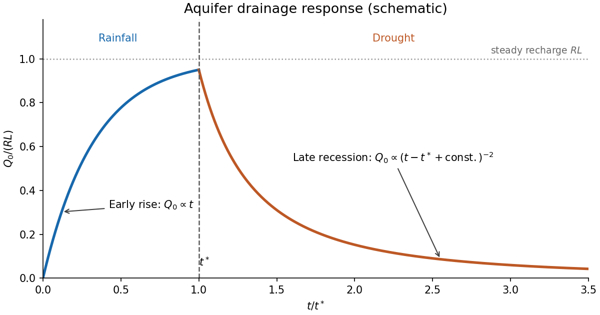
Let $J_X={\lim }_{x\downarrow 0}X(x)X^{\prime }(x)>0$. The spatial ordinary differential equation gives $(X{X}^{\prime }{)}^{\prime }=-\lambda X$, so its leading outlet behavior isAgain this is a square-root drainage boundary. For the separable aquifer drawdown, the dimensional drainage flux isEquivalently, with ${\tau }_d=\varphi /(K\lambda )$, it is $Q_0(t^{\ast })[1+(t-t^{\ast })/{\tau }_d{]}^{-2}$ for an exact separated profile. Integrating the spatial ordinary differential equation gives $J_X=\lambda {\int }_0^{L}Xdx$. This verifies the global mass conservation checkThus the late drainage flux follows an inverse-square power law, while stored water decays inversely with time.

The aquifer drainage hydrograph starts at zero, rises linearly in the early rainfall similarity solution, and approaches the total recharge $RL$ if rainfall lasts long enough for a finite-length steady state. Indeed, steady mass conservation gives $q_x=R$ and $q(L)=0$, hence $Q_0=RL$. At $t^{\ast }$, the outlet flux stays continuous for a regular inherited flux profile, then recedes as water drains; the eventual decay is proportional to $(t-t^{\ast }+\text{constant}{)}^{-2}$. An arbitrary transition requires the full time-dependent partial differential equation, so matching an early rainfall formula directly to a separated drought formula is only a schematic approximation.

The curve illustrates these regimes and a possible $t^{\ast }$. Its numerical shape and the relative duration of the regimes are schematic; the early rainfall and late drought formulas apply in their respective asymptotic ranges.