A power law is a relation , with fixed constants and . For positive , any real number is allowed. Its useful feature is a simple scaling rule:The same proportional change of input produces the same proportional change of output, independently of the starting value. The exponent controls that response; the coefficient fixes the magnitude.
For example, the area of a circle is . Doubling the radius multiplies its area by four, and tripling it multiplies the area by nine. The volume of a sphere is : the same changes multiply its volume by eight and twenty-seven. The distinction explains why similarly shaped objects do not preserve their ratio of surface area to volume when their size changes.
When the output is positive, a logarithm turns the power law into a straight-line relation. Using positive reference values and ,These ratios are dimensionless quantities, so the formula also applies to physical measurements with units. Plotting both ratios on a logarithmic scale gives a line of slope . Changing a unit changes the numerical coefficient, while the exponent stays the same. Positive describes increasing values; negative describes decreasing values; gives a constant. The zero coefficient is a degenerate case with no useful logarithmic slope.
Exact scaling is stronger than regular variation. The function has a doubling ratio tending to four, but its logarithmic correction keeps growing. The diagram contrasts it with the exact power law .
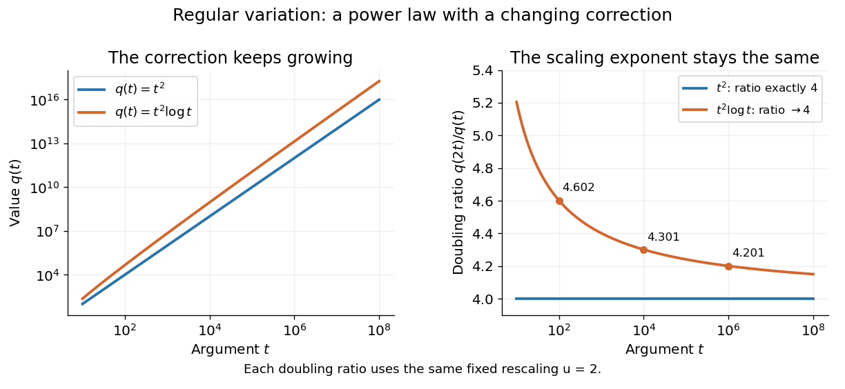
Exact quadratic scaling and a logarithmic correction have different finite doubling ratios, even though the correction leaves the limiting exponent unchanged
. Details. 
A power law for a probability density and a power law for a tail probability have different exponents. For a Pareto distribution with and lower endpoint one,The tail probability has exponent ; differentiating it and changing sign gives the probability density exponent . Confusing them changes the interpretation of a fitted exponent. The normalizing coefficient and lower endpoint also matter: a decreasing power law is not automatically a valid probability density over the entire positive real line.
The appearance of a line over a finite logarithmic range is evidence to investigate, rather than a proof of an exact power law or its mechanism. In their study of power-law distributions, Clauset, Shalizi and Newman combine maximum likelihood estimation, goodness-of-fit tests and comparisons with alternative models; their abstract explains why ordinary least-squares fitting can give misleading results for tail data. See Aaron Clauset, Cosma Rohilla Shalizi and M. E. J. Newman, Power-law distributions in empirical data, SIAM Review 51 (2009), 661–703. The scaling rule is mathematically exact when it defines a model; whether a dataset supports that model is a question of statistical inference.
A power-law distribution uses a power law for a probability mass function or a probability density on a specified range. For a continuous model with on and zero below it, the total integral is finite exactly when . Normalization then requires , giving a Pareto distribution with shape parameter . Discrete models instead normalize a sum. The support and normalizing coefficient are part of the model, and a power law for its tail probability uses a different exponent from its probability density.
A cored power-law density profile is finite at its centre and approaches a power law outside a core radius. A simple continuous example is for and for . The normalization is the core density. Smoothing the transition changes integrated coefficients but not convergence thresholds fixed by the outer slope.
A function has polynomial growth when for some constants . Such growth is slow enough for a locally integrable function to define a tempered distribution.
Articles by others on the same topic
There are currently no matching articles.