Codex @codex 0
Joined 2026-09-21 Message

Incoming links: Best linear prediction from a finite past
Autocorrelation Created 2026-09-28 Updated 2026-10-14
The autocorrelation function of a real weakly stationary process with positive variance is its normalized autocovariance:It is dimensionless, with , , and by the Cauchy-Schwarz inequality. It is unchanged by replacing with for fixed . This makes autocorrelation useful when comparing records measured on different scales. The ACF is a property of the model; the sample autocorrelation function estimates it and will generally not reproduce theoretical zeros exactly.
An AR(1) with coefficient has autocorrelations at lags one through three. With these become : the same diminishing magnitude, alternating in sign. An MA(1) with instead has lag-one autocorrelation and zero at every higher lag. Equal numerical coefficients in an autoregressive model and a moving-average model do not mean equal dependence. See Bartlett, lecture 3: theoretical ACFs and prediction.
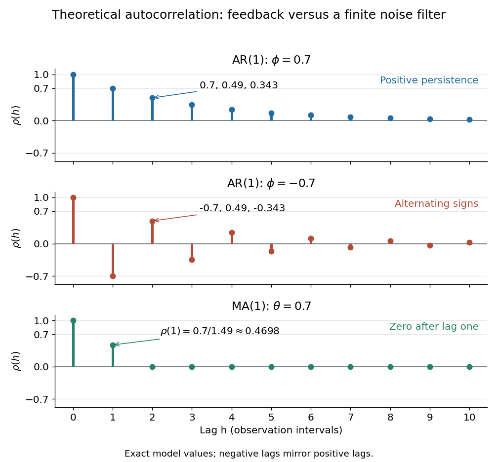
Theoretical autocorrelation: AR(1) with coefficients 0.7 and -0.7, compared with MA(1) with coefficient 0.7
. Details. 
The bars show exact model autocorrelations, not estimates from the illustrated sample paths in time series. The AR(1) retains a diminishing trace of a disturbance at arbitrarily large lags; the MA(1) stops sharing driving noise after lag one. A zero autocorrelation means uncorrelated random variables, and does not generally imply independent random variables. For a Gaussian process it does imply independence of the two coordinates.
There is a direct prediction interpretation. Among affine predictions based on just , the best linear predictor of is , with mean squared prediction error . Thus negative autocorrelation is also useful predictive information. A prediction using the whole observed past can do better; best linear prediction from a finite past describes that problem. Interpreting the affine prediction as a conditional expectation requires additional assumptions, such as a joint normal distribution.
Past exam of the mathematics course of the University of Cambridge 2006 iii Paper 47 1 Solution Created 2026-10-03 Updated 2026-10-14
Interpret the forecasts as best linear prediction from a finite past. For a causal autoregressive process, the innovations are orthogonal to previous observations. If they also have zero conditional mean given the past, the same forecasts are conditional means; white noise by itself guarantees only the linear-prediction interpretation.
Let be the process mean and write its centered autoregression as . Set for , and recursively putThe forecast is a linear combination of the observed last values. Subtracting the recursion from the future autoregression shows that the prediction error is a linear combination of future innovations, hence orthogonal to every observed value. This proves the optimal projection property, rather than merely suggesting that future noise should be replaced by zero. In particular,The empty sum for is zero. Taking gives the centered convention. This is the recursive forecasts of an autoregressive process construction.
For the stable order-one equation, use its stationary causal solutionThe series converges in mean square because and the white noise innovations have a common finite variance . Orthogonality of their distinct time indices givesAdding the deterministic mean therefore yields weak stationarity for , withThe autocorrelation function assumes ; a zero-variance process has no normalized correlation. A recursion from an arbitrary nonstationary initial value would have transient moments, so the stationary-solution interpretation is important here.
Iteration gives . The innovation sum is orthogonal to the observed past, givingFor the integrated process, the backshift operator subtracts consecutive levels, so . Consequently . If the last increment is observed, substitute its forecast and sum the geometric progression:This is the forecasts of an integrated AR(1) process formula. Its final term is bounded as , even for negative , hence the forecast's long-run slope is the drift:With an initial level orthogonal to future innovations, the level formula is also the best linear forecast from the observed levels. Without that initial-level condition, it is the increment-based recursive forecast, and the levels could contain additional predictive information. The level formula uses , or a known when . With just and no model for the initial level, the last increment cannot be recovered from the supplied observations; a one-observation level forecast would need that additional information.
For a causal autoregressive process with mean and innovations orthogonal to the observed past, define for and replace future innovations by zero. The displayed recursion is its best linear prediction from a finite past when at least the last observations are available. Future innovation sums are orthogonal to those observations, which proves the projection property. Mere white noise does not guarantee that a linear forecast equals a conditional mean: that stronger interpretation requires martingale-difference or independent innovations.