A time series is a sequence of observations indexed by time: hourly temperatures, daily sales, or successive measurements of a fluctuating signal. A probabilistic model treats these observations as one sample path of a stochastic process . For equally spaced observations, take and measure a lag of a time series in observation intervals. The order matters: shuffling a record preserves its observed values but destroys information about how one value follows another.
Two basic ways to model temporal dependence are an autoregressive model, which feeds past observations into the next value, and a moving-average model, which combines present and past white noise. An AR(1) carries a disturbance forward with diminishing weights; an MA(1) carries it into just two observations. Their autocorrelation functions make this difference visible. A weakly stationary process supplies a common mean and a lag-dependent autocovariance with which to describe that dependence.
These models help forecast future observations and quantify the uncertainty of averages. Successive measurements need not provide as much information as the same number of independent random variables: the long-run variance of a stationary process accounts for their accumulated covariances. Trend and seasonality require attention before fitting a stationary model; differencing and a seasonal difference operator can help, but do not automatically make every process stationary. See Peter Bartlett, Introduction to Time Series Analysis, lecture 1: objectives and models.
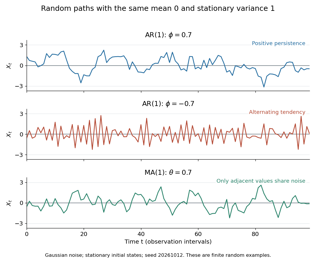
Stationary Gaussian examples: positive AR(1) persistence, negative AR(1) alternation, and MA(1) short memory
. Details. The three illustrated sample paths have zero mean and unit variance, so the visual comparison concerns dependence rather than scale. The AR(1) paths start from their stationary normal distribution, independently of future discrete Gaussian white noise; the MA(1) path includes the noise preceding its first observation. These are finite random examples, not exact pictures of an ACF. Compare their theoretical autocorrelation functions in autocorrelation.
Historically, Yule's 1927 study investigated disturbed periodicities in sunspot observations; it should not be read as the discovery of the particular AR(1) examples here. Slutsky studied how summing random inputs could produce wave-like records, a warning against inferring a periodic cause from appearance alone. The editorial note to his 1937 English paper identifies the 1927 Russian original. See G. Udny Yule, On a method of investigating periodicities in disturbed series, with special reference to Wolfer's sunspot numbers (1927) and Eugen Slutsky, The Summation of Random Causes as the Source of Cyclic Processes (1937), including the editorial note on the 1927 original.
A lag of a time series is a separation between observation indices. In an equally spaced time series, lag compares observations three intervals apart: for hourly readings this is three hours, while for daily readings it is three days. Positive and negative lags describe the same separation in opposite directions. The autocovariance and autocorrelation of a real weakly stationary process are even functions of lag.
A symmetric three-point smoother with weights reproduces constants only if . Reproducing quadratic trends also requires , so and . Thus the identity estimator is unbiased, but there is no nontrivial three-point linear smoother reproducing every quadratic. An assertion excluding even the identity estimator is false. This clarifies why the five-point symmetric quadratic trend smoother is the first symmetric nontrivial example.
For observations with a quadratic trend and uncorrelated equal-variance errors, a symmetric five-point linear filter of a stationary time series has weights . Reproducing every quadratic requires and . Substitution gives , and error variance . Its unique minimum occurs at , producing the displayed weights and variance . Negative weights are allowed: this is a linear weighted smoother, not a convex average. Applying a linear filter to a deterministic trend plus stationary errors does not assert that the complete observation process is stationary.
For independent identically distributed continuous observations, count strict local maxima and minima at interior positions. Each turning indicator has probability , adjacent indicators have joint probability , indicators two positions apart have joint probability , and more distant indicators are independent. Summing these covariances gives the displayed variance for . The indicators form a bounded 2-dependent sequence, giving an asymptotically normal standardized count. Too few turns suggests persistent trends; too many suggests alternation. Ties and dependent observations require a different calibration.
With a fixed gain , exponential smoothing recursively combines the newest observation with the preceding estimate. Iteration assigns geometric weights to older observations, together with a diminishing weight on the initial estimate. The steady-state local-level Kalman gain gives a probabilistic interpretation of this recursion.
Double exponential smoothing supplements a smoothed level with a smoothed slope so that forecasts can extrapolate a local linear trend. Two common versions are Holt's linear trend method, with separate level and slope gains, and Brown's double exponential smoothing, which applies the same smoothing gain twice. They are different algorithms, not two names for one recursion. Neither version by itself models seasonal variation.
For , set and . Use the displayed corrected level and slope, then forecast . For an exact linear trend after initialization transients, the first and second smooths have lags and twice that lag; their difference recovers the slope and the corrected level removes the lag. This is distinct from Holt's linear trend method.
Update the level and slope by and , with gains in . The first update compares the new observation with the previous level extrapolated one step; the second smooths the latest level increment. The displayed forecast extrapolates that local slope. This is a double exponential smoothing method for a nonseasonal trending time series.
For , update a local level by the displayed recursion and forecast every future horizon by . Iteration gives geometrically decreasing weights on past observations and a vanishing contribution from the initial level. It is useful for a locally stable level without a persistent trend or seasonality. A trend causes lag, motivating double exponential smoothing.
A second-order stationary time series decomposes into a deterministic component and a one-sided square-summable linear filter of a stationary time series of its mutually orthogonal linear innovations. Normalize . For a causal invertible ARMA process with no deterministic component, the driving white noise is this innovation process: observations and innovations span the same closed past subspace, while the next innovation is orthogonal to it.
The best mean-square linear predictor is orthogonal projection onto the span of the available centered observations, plus the known mean. Orthogonal innovations give a convenient basis of that span. Prediction at a future horizon must use only actually observed variables; it need not be a one-step predictor.
For a causal autoregressive process with mean and innovations orthogonal to the observed past, define for and replace future innovations by zero. The displayed recursion is its best linear prediction from a finite past when at least the last observations are available. Future innovation sums are orthogonal to those observations, which proves the projection property. Mere white noise does not guarantee that a linear forecast equals a conditional mean: that stronger interpretation requires martingale-difference or independent innovations.
If the increments of have mean and centered increments satisfy a causal autoregressive process of order one with , sum their recursive forecasts to obtain the displayed expression. For fixed forecast origin, . One must observe the last increment, requiring or a known initial level ; a single observed level without an initial-level model does not identify that increment.
Starting observations at a finite time, subtract the best linear predictor based on the available earlier observations. The resulting residual is orthogonal to their linear span. The unit-triangular relation between observations and residuals makes the residuals an orthogonal basis of the same finite observation space. These differ from infinite-past innovations until the initialization effect disappears.
In a centered MA(1) process, is uncorrelated with every observation through time . Its best linear predictor from that information is therefore zero, with error variance . One-step innovation formulas using cannot be substituted when that observation is unavailable.
Starting at time one, the orthogonal residuals satisfy , with and . Earlier innovation directions have zero covariance with the new observation. Explicitly, with , and for . These formulas follow by induction from , with and . This includes , where .
For an MA(1) process, the recursion has candidate limits and . The limit in is when and otherwise. The limiting innovation variance is , expressing the same covariance law through an invertible reciprocal representation.
The best mean-square linear predictor from a semi-infinite past is the orthogonal projection onto the closed linear span of past observations in the random-variable Hilbert space. For a causal invertible ARMA representation, past observations and past innovations generate the same closed span. The next linear innovation is orthogonal to it and is therefore the prediction error.
A state-space model separates a latent transition equation from an observation equation . A complete specification includes the initial-state law and its relation to the noise sequences, not just the two equations. Linear second-order models specify covariance structure; Gaussian versions additionally prescribe joint Gaussian laws.
For an autoregressive moving-average model of order , this state has observation row and transition matrixThe state noise is . Its first transition row reconstructs and its third row shifts the previous white noise value.
For and centered independent white noise values, the state above has expected value zero and this stationary covariance matrix, where . The cross-covariance with the future white noise value is zero and that with the contemporaneous white noise value is . Direct multiplication verifies .
The latent state follows a random walk, while observations add independent measurement noise. If the two noises have variances , the differences have autocovariances at lag zero, at lag one, and zero at larger lags. For , write and . The differenced process is an invertible moving-average model with coefficient and innovation variance . Its level has a unit root.
In a linear Gaussian state-space model, let the predicted state mean and covariance be . The observation innovation process has conditional mean zero and covariance , with innovation . The conditional multivariate normal distribution gives the predictive observation density. Multiplying these conditional densities by the chain rule gives the displayed likelihood function; equivalently the innovations are independent Gaussian vectors. The Kalman filter supplies recursively, so one evaluates the exact observed-data likelihood function without integrating all latent states jointly.
For , initialize the state by , with variance . It is orthogonal to future state noise and to observation noise orthogonal to all state noise. Under a Gaussian specification, take the initial state Gaussian with this variance and independent of future noises. Starting at zero instead gives a transient model.
An anticausal noise representation uses future rather than present and past innovations. For a two-sided AR(1) equation with , the stationary solution is . Thus stationary existence alone does not require causality.
A linear process is an L2-convergent white-noise filter , with square-summable coefficients. It is weakly stationary, and its autocovariance is . A causal representation restricts the coefficients to ; it is then an infinite moving-average representation.
When the transfer function is with distinct of modulus less than one, partial fractions give coefficients , where and . White-noise orthogonality gives covariance at lag as . This combines stable recursion with a closed geometric-sum covariance.
An ARCH model writes with standardized independent driving noise and a conditional variance . Typically and ensure a positive conditional variance. It allows a changing conditional scale even when is a stationary process.
With symmetric driving noise whose sign is independent of its magnitude, changing the sign of one driving variable changes the corresponding but leaves future conditional scales unchanged. Consequently for and square-integrable . This conclusion uses symmetry, beyond the martingale difference sequence property.
For and , the model splits into independent even-time and odd-time chains in its stationary causal solution. With standard normal noise, , and its fourth moment is finite exactly when .
The stationary squared process has the positive series . Even and odd observations therefore use disjoint families of independent random variables. This explains zero lag-one covariance of the squares despite dependence at lag two.
Volatility clustering means that large absolute observations tend to be followed by further large absolute observations, and small ones by small ones. In an ARCH process, persistence is in the conditional variance rather than necessarily in the signed observations.
Seasonality is systematic repetition at a calendar period. It can appear in a deterministic mean, in a periodic variance, or in dependence across seasons. A seasonal difference operator removes a fixed periodic mean but seasonal differencing does not remove periodic variance. A periodic-looking path alone does not prove a nonstationary process.
For an additive time series with period- seasonal component and , a centred average spanning one complete period removes the seasonal component while estimating the slowly varying trend. When is even, average two adjacent length- averages to centre the filter on an observation; the endpoints receive half the usual weights. Estimate each seasonal phase by averaging the corresponding detrended residuals across cycles, then subtract the mean of those phase averages to enforce the zero-sum convention. Multiplicative seasonality instead uses ratios and a mean-one convention. Repeated averaging is filter composition and induces serial dependence even from white noise.
A weakly stationary process can have very slowly decaying autocovariance, for example with and . Its sample mean can require a normalization different from . Long memory is dependence over long lags, rather than a changing marginal distribution.
In a second-order sense a weakly stationary process has short memory when its autocovariance is absolutely summable. Then its spectral density of a stationary process is continuous and its sample-mean variance has the usual finite long-run variance of a stationary process. A central limit theorem still needs additional conditions.
The difference can remove a unit-root stochastic trend. A seasonal difference operator instead subtracts an observation a full seasonal period earlier. Neither operation automatically removes a changing variance.
For an integer period , uses the backshift operator as . It annihilates a deterministic period- mean. If with and strong white noise, the result is the stationary moving average .
If with a deterministic periodic scale and strong white noise of variance , then . Its variance is , still seasonal when varies. A periodic scale model or variance standardization is more appropriate than blindly applying differencing.
An innovation measures the part of the current observation not predicted from past observations. The linear innovation process uses orthogonal projection onto the past linear span. A conditional expectation predictor can use nonlinear information; the two predictors agree for a Gaussian process.
Observe , with an independent Gaussian random vector of mean and covariance matrix . Its posterior is Gaussian with mean and covariance matrix . These formulas also hold for a singular positive semidefinite matrix . When is invertible, completing the square in the Bayes' theorem gives and . The observed innovation process is a Brownian motion in the observation filtration, and .
For the Gaussian Brownian drift filter with positive definite , define . Because and , the Itô formula gives . Thus is a positive stochastic exponential, hence a nonnegative local martingale and a supermartingale. For a singular prior, the inverse-matrix expression is undefined; the same process can instead be defined by , with treated as fixed inside this Gaussian integral.
For the Gaussian Brownian drift filter , with independent prior , the observation law has densityrelative to driftless Wiener measure. The law having fixed observation drift has density relative to the same reference. Their ratio is therefore a positive mean-one density on every finite horizon. In the observation filtration it satisfies , where is the posterior mean and the innovation process. This density-ratio argument establishes a true martingale without an unsupported global Novikov condition for the unbounded posterior mean.
For and fixed , subtracting leaves the Brownian bridge . It is independent of , since it is independent of and has zero covariance with in their jointly Gaussian law. The observed path is determined by this bridge and its endpoint, so the bridge gives no further information about . Hence conditioning on the full observation filtration at gives the same posterior as conditioning on alone.
For with an independent equiprobable drift , the likelihood ratio between the two drifts is . Multiplying the normal distribution densities of successive increments proves this ratio for every observation partition; continuity then gives the full observed-path posterior. The Bayes' theorem gives . Thus the observed drift is . The process is an observed-filtration martingale with quadratic variation , so the Lévy characterization of Brownian motion makes it a Brownian motion. The observed state is a scaled diffusion with hyperbolic tangent drift.
For a square-integrable time series, let be the closed linear span of its past. The innovation is orthogonal to every past linear observation. A causal invertible autoregressive moving-average model is driven by these innovations, which are weak white noise for a weakly stationary process.
A naive forecast repeats the latest observation at every future horizon. For a stationary mean- process its horizon- mean squared prediction error is . A forecast of the known mean has risk , so persistence is not automatically better when lagged dependence is weak.
A causal time series can be expressed using present and past innovations, without future innovations. The autoregressive process of order one with has the mean-square convergent causal representation .
A causal time-series representation expresses a time series using present and past driving white noise. Its coefficients vanish at negative lags. Square summability ensures mean-square convergence for a white-noise input; absolute summability is the stronger stable-filter convention. Causality refers to the particular driving sequence, not merely to stationary existence.
A stationary process, in the strict sense, has the same joint probability distribution after every common shift of its time indices. More precisely, for every positive integer , every choice of times , and every integer shift ,Here equality means equality of probability distributions, not equality of realized observations. A sample path can fluctuate, stay positive for a while, or show accidental runs while its generating law remains stationary. Strong white noise is a basic example: shifting time preserves every joint law of its independent and identically distributed random variables.
The distinction between strict stationarity and weak stationarity is useful. The former preserves all finite joint laws; the latter preserves only the finite mean and covariance structure. Strict stationarity with finite second moments implies weak stationarity, but strict stationarity itself does not require finite variance. A Gaussian process with weak stationarity is also strictly stationary, because each of its finite-dimensional distributions, a joint normal distribution, is determined by its mean vector and covariance matrix.
Every finite-dimensional distribution of a strictly stationary process is invariant under a common shift of its time indices. If second moments are finite, strict stationarity implies a weakly stationary process. A constant mean and lag-dependent covariance alone do not imply strict stationarity.
Let and be the sigma-algebras generated by the past and future observations. The mixing coefficient is . Strong mixing means . Appropriate quantitative mixing and moment conditions can imply a central limit theorem; absolute summability of autocovariance alone does not.
A stationary path law is ergodic when every time-shift-invariant event has probability zero or one. The Birkhoff ergodic theorem then identifies integrable time averages with deterministic ensemble expectations. A shared random scale multiplying iid noise gives a stationary counterexample: it is uncorrelated across distinct times, but the path retains information about the random scale.
A process is nonstationary if some finite-dimensional distribution changes under a common time shift. With finite second moments, failure of a constant mean or variance, or failure of lag-only covariance, already rules out a weakly stationary process. A periodic mean or periodic variance can instead give a periodically correlated process.
A real stochastic process is a weakly stationary process if it has finite second moments, a constant expected value , and an autocovariance depending only on the lag of a time series:In particular its variance is the same at every time, . This is often called second-order stationarity. It makes observations from different parts of a record comparable through the same autocorrelation function. Bartlett uses this second-order meaning of stationarity in Introduction to Time Series Analysis, lecture 2: mean, covariance, and stationarity.
For a worked contrast, let be centered white noise of variance . The process has mean , variance , and zero autocovariance at nonzero lags, so it is weakly stationary. The process has exactly the same covariance structure, but its mean is , so it is not weakly stationary. Constant variance alone is insufficient.
Weak stationarity need not imply strict stationarity. For example, choose independent random variables at all integer times, using a standard normal distribution at even times and a Rademacher distribution at odd times. Every coordinate has zero mean and unit variance, and distinct coordinates have zero covariance. Nevertheless a shift by one changes the marginal probability distribution from continuous to two-point. This also illustrates why weak white noise need not be identically distributed.
An absolutely summable sequence of coefficients defines in mean square. It remains weakly stationary and has covariance . Its frequency response is .
For absolutely summable linear-filter coefficients, the generating function is the displayed Laurent series, absolutely convergent on the unit circle. If the filter is one-sided, it is a power series analytic inside the unit disk. A two-sided filter need not have a nonempty larger annulus of convergence. Substituting the backshift operator gives the formal notation .
The transfer function is the filter generating function evaluated on the unit circle, with a sign convention matching the Fourier representation. Filtering a sinusoid of angular frequency multiplies its complex amplitude by . Its modulus is the filter gain; filtering a weakly stationary process multiplies its time-series spectral density by . Using the opposite Fourier sign conjugates the response for real coefficients and leaves that squared modulus unchanged.
Two absolutely summable linear filters of a stationary time series compose by convolution: and . Absolute convergence in the space of square-integrable random variables justifies exchanging the sums. The frequency responses multiply, giving the spectral density transformation under a linear filter twice.
For an absolutely summable linear filter of a stationary time series, the filter gain is the modulus of its frequency response . It multiplies a sinusoidal amplitude, while its square multiplies the spectral density of a stationary process. A zero removes the corresponding frequency; the filter gain of a composition is the product of the two filter gains.
Filtering multiplies the time-series spectral density by the squared modulus of the frequency response. Insert the spectral integral into the covariance double sum and interchange sums using absolute summability of the filter. This holds even when the input covariances are not absolutely summable, provided the spectral measure has a density.
The symmetric filter with weights has unit gain at zero frequency, but its largest gain is at signed frequencies . Applied times, it multiplies a spectral density by . Thus repetition amplifies and selects a period-six oscillation instead of merely suppressing short-scale noise. On a two-sided frequency domain both peaks must be retained.
The spectral measure of a weakly stationary process is the finite nonnegative measure whose Fourier coefficients are its autocovariances. Its total mass is the process variance. A time-series spectral density exists exactly when this measure is absolutely continuous with respect to Lebesgue measure.
For uncorrelated zero-mean unit-variance amplitudes , the process has covariance and hence the displayed two-atom spectral measure of a stationary time series. Independence or Gaussian amplitudes are unnecessary for weak stationarity. A phase shift need not preserve the whole joint amplitude distribution, so strict stationarity cannot be inferred from these second moments alone.
The cumulative function of the finite positive spectral measure of a stationary time series is nondecreasing and right-continuous, with total mass equal to the variance. For an absolutely continuous measure, , where is the time-series spectral density. Under angular-frequency normalization, and, when the covariance series is absolutely summable, . Atoms describe persistent periodic components and cannot be represented by an ordinary density.
A second-order stationary complex random field on the line has uncentered correlation . When this correlation is continuous, its Fourier transform is a finite positive measure characterized by . Its total mass is . If it has a density, . A constant mean contributes ; the remaining measure is the covariance spectrum. This uncentered convention is useful for coherent and diffuse wave fields.
For the Fourier transform of a stationary random field, the periodogram measure converges weakly to the spectral measure of a stationary random field. The expected squared modulus is . The factor follows from Parseval identity, and preserves the total power per unit length. It also avoids meaningless squares of Dirac delta distributions for coherent plane-wave components.
With absolutely summable autocovariance, the asymptotic variance of the sample mean satisfiesThe sum is signed, rather than a sum of absolute values. It can be zero: the first difference of strong white noise has telescoping partial sums. A central limit theorem needs further dependence assumptions.
When the long-run variance of a stationary process is positive, matching the variance of its average to an average of independent observations gives . Positive aggregate correlation reduces this size; negative aggregate correlation can increase it beyond the observation count. This extends the variance interpretation of effective sample size of a Markov chain.
When its autocovariance is absolutely summable, a weakly stationary process has spectral density . The inverse relation is . A linear filter multiplies this density by the squared modulus of its frequency response.
Under angular-frequency normalization, the displayed time-series spectral density gives and for nonzero integer . This follows from the even integral . All nonzero even-lag covariances vanish while the odd-lag covariances are positive.
For zero-mean real weakly stationary processes whose cross-covariances are summable, the cross-spectrum is the Fourier series of their lagged covariance, with the displayed convention. Reality gives , but the cross-spectrum need not be real or even. Exchanging the two series gives . The entries form a Hermitian spectral density of a stationary process matrix.
For real stationary processes, the one-sided density on is twice the usual two-sided density. Its integral is the variance and . When covariances are absolutely summable, .
For a real weakly stationary process, restricting its even angular-frequency density to gives . Folding both frequency halves into one density gives and removes that factor two. Consequently white noise of variance has restricted density and folded density .
A weakly stationary process has a time-series spectral density precisely when its spectral measure of a stationary time series is absolutely continuous with respect to Lebesgue measure. Absolute summability of its autocovariances is sufficient and yields a continuous Fourier-series density. It is not necessary for existence; for a general integrable density, Fejér sums give an recovery formula.
In cycles per observation, frequency lies in and . Compared with angular-frequency density , one has . In particular, white noise of variance has .
A centered weakly stationary process has a representation with orthogonal random increments. Their variance measure is the spectral measure. When it has density , the autocovariance is .
For a centered record of length , the periodogram is the squared modulus of its discrete Fourier transform, with normalizationUnder suitable short-memory assumptions its expectation approaches the spectral density of a stationary process, but its variance generally does not vanish. Smoothing nearby frequencies can provide an estimate with statistical consistency.
At an interior frequency, the real and imaginary Fourier coefficients of a short-memory Gaussian time series converge jointly to independent centered normal variables, each with variance , where is the one-sided spectral density. Their squared sum therefore converges to . Its variance tends to , so an unsmoothed periodogram is not consistent when . Averaging nearby ordinates can reduce this persistent variance.
For a centered stationary real Gaussian sequence, let and be its cosine and sine coefficients with normalization at a nonzero Fourier frequency. Grouping the double covariance sum by lag and extending each lag sum to a whole record leaves at most omitted bounded products. The full cosine-sine sum is zero, giving the bound. If , the two coefficients become asymptotically uncorrelated, and their limiting joint normal distribution consequently has independent components.
Average neighboring periodogram ordinates with nonnegative weights summing to one. Let the number of averaged ordinates tend to infinity while their frequency span, of order , tends to zero. For a smooth spectral density and suitable short-memory or fourth-order dependence conditions, the bias tends to zero and variance is of order . Smooth second-order spectral density alone does not ensure this: a time-constant random scale multiplying independent white noise has a smooth unconditional spectrum but a nonergodic random limiting local power.
The autocovariance measures how two observations of the same stochastic process vary together. For a real weakly stationary process of mean , it isWeak stationarity removes dependence on the absolute time . Without it, the covariance function generally needs two time arguments. Lag zero is the variance, ; symmetry of real covariance gives . Positive values favor deviations from the mean in the same direction; negative values favor opposite directions. The units are the square of the observation units. See Bartlett, lecture 2: autocovariance examples.
For example, if with centered unit-variance white noise, expanding the product leaves only matching noise times. Thus , , and for . This MA(1) has a positive lag-one autocovariance because adjacent observations share one disturbance. Rescaling every observation by multiplies every autocovariance by , while leaving autocorrelation unchanged.
The autocovariance is useful beyond comparing pairs: it determines the variance of any finite linear combination of observations. For the sample mean ,Each separation occurs in pairs. For the preceding MA(1) and , this is , compared with for four uncorrelated random variables of the same variance. This is the finite-record counterpart of the long-run variance of a stationary process.
For a known zero mean, for . Weakly stationary process assumptions give expectation . Dividing by instead gives an unbiased estimate at each individual lag, although the resulting collection need not form a positive semidefinite covariance sequence.
The autocorrelation function of a real weakly stationary process with positive variance is its normalized autocovariance:It is dimensionless, with , , and by the Cauchy-Schwarz inequality. It is unchanged by replacing with for fixed . This makes autocorrelation useful when comparing records measured on different scales. The ACF is a property of the model; the sample autocorrelation function estimates it and will generally not reproduce theoretical zeros exactly.
An AR(1) with coefficient has autocorrelations at lags one through three. With these become : the same diminishing magnitude, alternating in sign. An MA(1) with instead has lag-one autocorrelation and zero at every higher lag. Equal numerical coefficients in an autoregressive model and a moving-average model do not mean equal dependence. See Bartlett, lecture 3: theoretical ACFs and prediction.
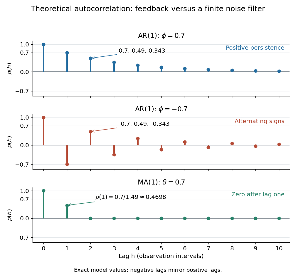
Theoretical autocorrelation: AR(1) with coefficients 0.7 and -0.7, compared with MA(1) with coefficient 0.7
. Details. The bars show exact model autocorrelations, not estimates from the illustrated sample paths in time series. The AR(1) retains a diminishing trace of a disturbance at arbitrarily large lags; the MA(1) stops sharing driving noise after lag one. A zero autocorrelation means uncorrelated random variables, and does not generally imply independent random variables. For a Gaussian process it does imply independence of the two coordinates.
There is a direct prediction interpretation. Among affine predictions based on just , the best linear predictor of is , with mean squared prediction error . Thus negative autocorrelation is also useful predictive information. A prediction using the whole observed past can do better; best linear prediction from a finite past describes that problem. Interpreting the affine prediction as a conditional expectation requires additional assumptions, such as a joint normal distribution.
A correlation time measures how rapidly a stationary stochastic process loses temporal dependence. Specify whether it means an exponential decay time, an integral of the normalized autocorrelation, or another width. For , the exponential time and the one-sided integral both equal .
The partial autocorrelation at lag is the correlation of and after their linear projections onto the intervening observations are removed. A causal autoregressive model of order has zero partial correlations after lag . This complements the finite cutoff of the autocorrelation function for a moving-average model.
Replace the autocovariance in the finite-lag linear prediction equations by the sample autocovariance function. The last regression coefficient at order estimates the lag- partial autocorrelation function.
The sample autocorrelation function replaces the mean and lagged covariance in by their empirical counterparts.
A correlogram plots the estimated autocorrelation function against lag. The plot helps distinguish the finite autocorrelation cutoff of a moving-average model from the decaying dependence of a causal autoregressive model. Estimated cutoffs are diagnostics, not exact finite-sample identities.
For the AR(1) and MA(1) formulas here, white noise means a real sequence indexed by all integer times withThese are the weak white noise assumptions: zero mean, a common finite positive variance, and uncorrelated random variables at distinct times. Independence and a normal distribution are additional assumptions. Strong white noise requires independent and identically distributed random variables; discrete Gaussian white noise is the jointly Gaussian special case. Some definitions allow a constant nonzero mean; subtract it before using the centered formulas here.
For a concrete dependent example, let equal or with equal probabilities, independently of a sequence of independent Rademacher random variables , and put . Its mean is zero, its variance is , and its nonzero-lag autocovariances vanish. Nevertheless every equals the same : seeing one magnitude determines all the others. This is white noise with dependence invisible to its ACF, and is also an example of the issue discussed in ergodic stationary process.
Discrete Gaussian white noise is a jointly Gaussian sequence with expected value zero and covariance at lag zero and zero at other lags. Joint normality makes the components independent. This is a sequence of ordinary random variables, unlike the generalized continuous-time white-noise process.
Continuous-time Gaussian white noise is a random distribution rather than an ordinary finite-variance function at every time. Integrating it against deterministic kernels gives Gaussian random variables with covariance . For independent isotropic components, a three-dimensional dot covariance has amplitude . An ordinary rapidly decaying force covariance approximates this model only above its correlation time.
A sequence of independent and identically distributed random variables with zero mean and finite variance is strong white noise. It is weak white noise, but need not have a normal distribution.
A white noise sequence has zero mean, a common finite variance and zero autocovariance at every nonzero lag. This requires uncorrelated random variables, rather than independent random variables.
An autoregressive–moving-average model satisfieswhere is the backshift operator, and are finite polynomials, and is white noise.
For a causal autoregressive moving-average model driven by independent white noise, multiply its recursion by and take covariance. When , all driving white noise values in its moving-average term occur strictly after , so their covariances with vanish. The resulting homogeneous tail recurrence has the same characteristic roots as the autoregressive model recursion. Distinct roots of modulus below one give exponential autocovariance decay.
Normalize the autoregressive and moving-average polynomials to have constant coefficient one, cancel common factors, and require all their zeros to lie outside the closed unit disk. With positive innovation variance these conditions give a causal, invertible, minimal Gaussian process representation. To prove identifiability, compare two such models with the same time-series spectral density. The ratio of their scaled rational transfer functions and its reciprocal are analytic on a neighbourhood of the closed unit disk and have modulus one on its boundary. The maximum modulus principle makes the ratio constant; its positive value at zero forces equality of the innovation variances and equality of the rational functions. Coprimality and the constant-coefficient normalization then force equality of both polynomials. Without the root restrictions, reciprocal root reflection of an ARMA representation and a rescaling of the innovation variance can preserve the spectrum, so the unrestricted parameters are not identifiable.
An ARIMA model applies an autoregressive moving-average model to the differenced process , where is the backshift operator. Differencing permits stochastic trends whose levels are not weakly stationary processes. A local random-walk level observed with independent measurement white noise has an ARIMA(0,1,1) representation, or a formal ARMA(1,1) equation with autoregressive coefficient one.
For an autoregressive moving-average model, set and . If both have no zeros on the closed unit disc, the causal and inverse filters have absolutely summable coefficients and . Comparing power series coefficients gives and , where , for , and all out-of-range coefficients vanish. The backshift operator then gives the corresponding time-series filters.
Articles were limited to the first 100 out of 154 total.
Articles by others on the same topic



A time series is a sequence of data points recorded or measured at successive points in time, typically at uniform intervals. It is a common method in statistics and various fields, such as finance, economics, environmental science, and engineering, for analyzing trends, patterns, and behaviors of data over time. Key characteristics of time series data include: 1. **Temporal Order**: The data points are ordered chronologically. Each observation has a timestamp, and the order matters.