The variance measures the mean squared distance of a random variable from its expected value. For a real square-integrable random variable ,The square prevents positive and negative deviations from cancelling. It also gives the variance squared units: if measures a length in metres, its variance has units of square metres. Its nonnegative square root is the standard deviation, which has the same units as .
For example, let take , and with equal probabilities. Its expected value is zero, but its variance is , and its standard deviation is . The constant random variable zero has the same expected value and zero variance: a mean alone does not describe the spread. The variance is zero exactly when almost surely.
The variance is useful because squared deviations interact neatly with linear combinations. The covariance supplies the cross terms when combining different random variables, and a covariance matrix organizes those terms for many variables. The characterization of variance as the minimum mean squared error of a constant also explains why the expected value is the best constant prediction under squared error.
For independent identically distributed random vectors with finite second absolute moments, expand . Their independence makes , proving the identity. The right side is the sum of the coordinate variances. Applied to the displacement in an optimal transport plan, it separates motion of the barycenter of a measure from relative particle motion.
For a finite population with arithmetic mean , its variance is . It averages squared deviations over the whole population.
For a nonnegative count with positive mean, the Fano factor compares its variance to its mean. A Poisson distribution has factor one. Correlated production bursts or weak restoring feedback can give factors larger than one even at large molecular copy number.
// Target: mathematical-biology.bigb
For a square-integrable real random variable ,Thus the unique best constant predictor is , and the minimum mean squared error is .
The conditional variance measures the remaining squared uncertainty after specified information has been used to form a conditional mean. For a real square-integrable random variable and a sub-sigma-algebra , let . ThenIt is a -measurable random variable, nonnegative almost surely, rather than necessarily a single number. With the information , its value is the variance in the group identified by . Its expected value is the mean squared error of predicting by its conditional mean.[ref]
In the exact mixture distribution in law of total expectation, group contains around mean two, and group contains around mean eight. Both groups have conditional variance four because their deviations from their own means are with equal probabilities. Therefore . Meanwhile, the two group means have variance . The law of total variance givesDirect calculation gives and , checking the decomposition.
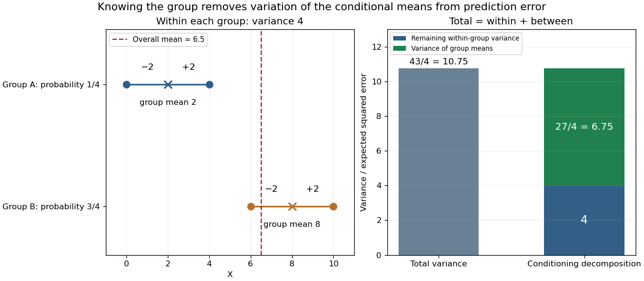
For any square-integrable -measurable predictor , the error identity isThe cross term vanishes because . Thus using the conditional mean minimizes mean squared error, while conditional variance quantifies what this information still cannot predict. This is the orthogonal projection interpretation in L2 space.[ref]
For square-integrable and nested information , let and . The predictor is also -measurable, so the conditional variance error identity givesMore information cannot increase the average best squared prediction error. Equality holds exactly when the two conditional means agree almost surely; additional information can change the conditional distribution without changing its mean.
This is an averaged statement. Take with equal probabilities, and learn only whether is zero. The unconditional variance is . In the nonzero group, the conditional variance is , which is larger; in the zero group it is zero. Their weighted average remains . Both groups have conditional mean zero, so the extra information has not improved squared-error prediction, even though it has revealed whether the outcome is extreme or central. An individual group's conditional variance need not decrease.
For independent random variables with , writeThen . Hence converges in exactly when the scalar Cesàro means converge.
Let each be uniform on , with arbitrary dependence. For centered unit-norm , putThenPartition into equal intervals and test normalized differences of two interval indicators. Averaging over the two intervals reduces the claim to for their occupancy counts, and then let .
The covariance measures the average product of two centered deviations. For real square-integrable random variables and ,Deviations with the same sign contribute positively; deviations with opposite signs contribute negatively. Their magnitudes and probabilities determine the net result. Taking recovers the variance. The definitions and algebraic properties are presented in Orloff and Bloom, MIT 18.05, Covariance and Correlation, sections 2–2.1.
For a worked example, let be independent random variables, each equally likely to be , or , and put . All nine pairs have probability . The expected values are zero, while linearity of covariance and the vanishing covariance of independent random variables giveThe shared term makes large accompany large on average. Replacing by reverses the covariance to without changing either variance.
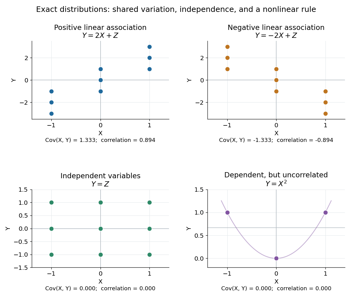
Positive, negative, independent, and nonlinear relationships have different covariance behavior
. In the first three panels, and independently take , and with equal probabilities; each point has probability . In the last panel, , and the three marked outcomes each have probability . The thin curve shows that quadratic function. Its zero covariance leaves strong nonlinear statistical dependence visible. Details.The covariance is useful whenever deviations are added or subtracted. Expanding the square givesFor the worked model, these are and . Positive covariance increases variation in the sum while reducing variation in the difference: the same shared fluctuation reinforces one combination and partly cancels in the other. The identity applies beyond independent random variables.
The size of a covariance depends on the measurement scale. For constants , linearity of covariance gives . Adding offsets has no effect; rescaling either measurement rescales the covariance. The Pearson correlation coefficient divides by both standard deviations to describe the standardized linear relationship.
Two random variables have negative covariance when , assuming finite second moments. Opposite deviations from their respective expected values then outweigh matching deviations on average. For example, if for a constant , the bilinear identities of covariance give , which is strictly negative when has positive variance.[ref]
Covariance and Correlation by Jeremy Orloff and Jonathan Bloom. §2.1, scaling and covariance with oneself
Sampling without replacement gives a useful example in which the negative sign comes from a shared finite resource. Choose a simple random sample of exactly distinct members from a statistical population of size , with . For each member define the inclusion indicator . Its inclusion probability is . For different members , the joint inclusion probability isSubtracting the product of the expected values givesThe Pearson correlation coefficient follows because each inclusion indicator has variance . Once member is included, only places remain for the other members, reducing member 's conditional probability of inclusion below .
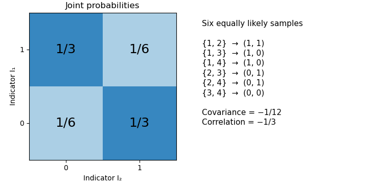
For an original exact example, draw two members from four. The six unordered sample pairs are equiprobable. For , the outcomes and each have probability , while and each have probability . Hence , and their Pearson correlation coefficient is . Matching outcomes remain possible despite the negative covariance.
A fixed total alone does not force every pair among three or more random variables to have negative covariance. If , thenThis constrains the sum of the off-diagonal entries in a row of the covariance matrix. It does not fix each entry's sign. For a counterexample, let be equally likely to be zero or one, and set , , . Their total is always two, yet .
In the simple random sample, exchangeability makes the off-diagonal covariances equal, so the fixed-total identity does determine each of them: . The same distinction between a linear constraint and individual pair signs matters for the joint dependence of leave-one-out consensus residuals.
Two random variables have positive covariance when their centered product has positive expected value:Assume throughout that their second moments are finite. Outcomes where the centered values have the same sign contribute positively; opposite signs contribute negatively. The sign describes their average balance, rather than requiring every outcome to have matching signs.[ref]
Covariance and Correlation by Jeremy Orloff and Jonathan Bloom. §§2–2.1, definition and properties of covariance
A shared group effect can produce positive covariance even when the relation inside each group runs in the opposite direction. For an exact original example, let and be independent random variables with the Rademacher distribution: each takes the values with equal probability. Define and . Both expected values vanish, and independence givesTheir Pearson correlation coefficient is consequently . The four equiprobable outcomes are , , and .
For either fixed value , however, . Thus the conditional covariance is , and the conditional Pearson correlation coefficient is : the two points inside each group lie on a descending line. The law of total covariance identifies exactly where the positive pooled value comes from:The first term averages the conditional covariances; the second measures how the two conditional expectations move together across groups. Here the between-group contribution outweighs the negative within-group contribution. This is a covariance form of Simpson's paradox.
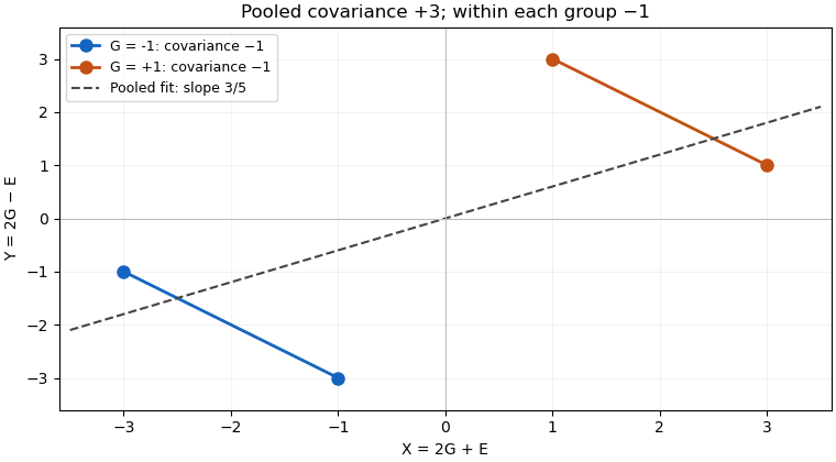
The dashed linear regression line has slope , but that slope does not give the direction of the relation at fixed . Nor does positive covariance by itself establish a causal effect: in the specified model the common variable supplies the positive component. Choosing which variables to condition on is a question about the model and the intended comparison, beyond computing one number.
Positive covariance is also weaker than requiring one variable to be an increasing function of the other. Under appropriate integrability assumptions, strict positive covariance with an increasing payoff supplies a useful sufficient condition; the grouping example shows a different route to the same sign.
For mutually independent square-integrable random variables , factor the joint moment as , then subtract the product of the two means. This proves the formula. Sharing one factor can therefore produce nonzero covariance even when all original factors are independent. Products of disjoint groups of independent factors are themselves independent random variables.
For square-integrable random variables, expand and into their conditional expectations and their centered conditional residuals. The cross terms vanish by the law of total expectation, giving the displayed covariance decomposition. conditional independence can therefore coexist with positive unconditional covariance from a shared latent variable.
Let be a nondegenerate real random variable and a strictly increasing function. Assume , and are integrable. For an independent copy ,The product is positive whenever and zero otherwise. Nondegeneracy gives positive probability of unequal copies, proving strict positivity. The same argument applies to a conditional distribution when that conditional law is nondegenerate and has the required integrability.
For a market with one trading period, suppose an increasing terminal payoff is replicated by a risk-free asset holding and a stock holding: . Under current information , let be -measurable and . ThenThis is a conditional one-period statement. General dynamic attainability alone does not specify the affine representation used in this calculation.
For square-integrable random variables, . It is a -measurable random variable. Replacing by its conditional expectation given a larger sigma-field leaves this covariance unchanged when is measurable with respect to that larger sigma-field. This observation underlies recovery of a martingale-transform integrand by conditional covariance.
For paired observations , the sample correlation coefficient isIt is the normalized inner product of the centered data vectors, or the sample covariance divided by the product of the corresponding sample standard deviations. The choice of divisor or cancels when used consistently in all three quantities. It is undefined if either centered data vector is zero, which occurs when that variable is constant in the observed statistical sample.
For and , both sample means are . The sum of centered products is , and each sum of centered squares is , hence the sample correlation coefficient is . This is a summary of these four observed pairs; it is not automatically the population Pearson correlation coefficient. Philip Stark, Computing the correlation coefficient explains the centered and standardized calculation.
A sample correlation matrix rescales a sample covariance matrix to unit diagonal, for variables with positive sample variance. Its off-diagonal entries are sample correlation coefficients. Strong correlations between predictors can indicate multicollinearity, but pairwise correlations alone do not exclude higher-order linear dependence.
For square-integrable complex random variables, the Hermitian covariance is . Its diagonal is nonnegative and equals . The conjugation distinguishes it from the pseudo-covariance.
For a centered complex random variable , the pseudo-covariance is . Together with it determines the real covariance matrix: , , and .
For independent standard normal random variables , define the displayed errors for . Each has mean zero and variance one. Nonadjacent errors depend on disjoint sets of independent variables. Adjacent covariances vanish because their product contains an independent centered factor. Thus their covariance matrix is .
They are nevertheless dependent: the Gaussian fourth moment gives , and hence . Constant variance and zero pairwise covariance can conceal dependence in magnitudes. This is useful when interpreting a residual plot in linear regression.
For two Bernoulli random variables with joint probabilities in the order , their covariance is . Zero covariance fixes the probability to the product of its marginals; subtracting this from each marginal fixes all three remaining joint probabilities to their products. Thus uncorrelated random variables taking only zero and one are independent, including degenerate marginals. The implication is special to this two-point setting and fails for general distributions.
For a real random vector with finite second moments, its covariance matrix collects all pairwise covariances:The diagonal entries are variances. The covariance matrix is a symmetric matrix and a positive semidefinite matrix, because for every real vector ,Thus one matrix describes the variance of every linear combination of the coordinates. It is a positive-definite matrix exactly when no nonzero linear combination is constant almost surely. A deterministic linear relation produces a zero eigenvalue.
For example,has unit coordinate variances, covariance , and eigenvalues and . Its unit eigenvectors and describe directions of greatest and least projected variance. For a unit vector , direct multiplication gives : the variation in the sum direction is nine times that in the difference direction.
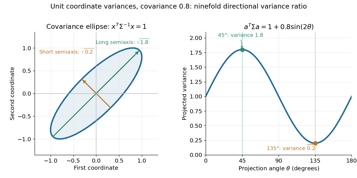
The spectral theorem supplies an orthonormal basis of these directions. This connects covariance matrices to principal component analysis: its leading eigenvector identifies the unit-direction projection with the largest variance. For a linear transformation , the transformed random vector has covariance matrix , so uncertainties propagate through a linear model by matrix multiplication.
Every real symmetric matrix satisfying for every real vector is the covariance matrix of a random vector taking only finitely many values. The stated inequality means that is a positive semidefinite matrix. One does not need a multivariate normal distribution to realize a specified second-moment geometry. Conversely, a proposed covariance matrix must be positive semidefinite, since is the variance of the projection onto any real vector .
Here is an explicit construction. If is the matrix rank of , orthogonal diagonalization gives a real matrix withLet be independent Rademacher random variables, each equal to or with probability , and put . Then and , soThe random vector has at most possible values. Adding any constant vector prescribes its mean without changing its covariance matrix. If , the constant vector alone suffices.
For an original two-dimensional example chooseThe four equally likely values of areTheir coordinate means vanish. Their squared first coordinates average to , their squared second coordinates to , and their coordinate products to . The displayed covariance matrix is therefore realized exactly, without sampling error or an asymptotic argument.
These four values are a complete probability model with masses , not automatically an independent random sample whose population is unknown. Applying the usual divisor-three sample covariance matrix to the same four rows would give . NIST explicitly distinguishes that unbiased sample formula with divisor ; probability-weighted population moments use the assigned masses instead.[ref]
NIST and SEMATECH e-Handbook of Statistical Methods. Section6.5.4.1, Mean Vector and Covariance Matrix, unbiased sample formula
The sign construction need not minimize the number of points. If a distribution has positive-mass support points, the centered points obey one nontrivial weighted relation, so their span has dimension at most . Its covariance matrix consequently has matrix rank at most , requiring when . Matching a covariance matrix also does not match the full probability distribution: this finite model and a continuous Gaussian model can have identical means and covariances while assigning very different probabilities to nonlinear events.
For real random vectors and with finite second moments, their cross-covariance matrix collects the covariances between the two sets of coordinates:It has size , and exchanging the two vectors transposes it: . Unlike a covariance matrix of a vector with itself, a cross-covariance matrix need not be square or symmetric.
For an original construction, let centered independent random variables have variances1and4, and putLinearity of covariance givesThe second entry contains a negative contribution from , although the total is positive. Also andThis joint covariance matrix is positive semidefinite. That restriction couples its diagonal and off-diagonal blocks; an arbitrary rectangular matrix cannot be combined with arbitrary within-vector covariances to produce a valid joint model.
For fixed real matrices and constant vectors , direct substitution into the definition givesThis identity propagates shared input fluctuations through two different linear readouts, for example when assessing shared calibration error.
From independent identically distributed paired observations, the usual unbiased estimate isThe pairing must be preserved: independently shuffling the second set changes the estimated association. NIST's multivariate tutorial gives the coordinate sample-covariance formula and its assembly into a covariance matrix; the rectangular formula above is the block joining the two chosen coordinate groups.[ref]
For a two-dimensional positive-definite covariance matrix , the centered covariance ellipse is the image of the unit circle under its positive definite square root of a matrix. Equivalently, it satisfies . Its semi-major and semi-minor axes have lengths given by the square roots of the larger and smaller eigenvalues, along the corresponding eigenvectors. The ellipse encodes a second-moment geometry; a probability-coverage interpretation needs additional information about the probability distribution and the chosen scale.
For a random vector with covariance and positive coordinate variances, let . Its correlation matrix is the covariance of , so it is positive semidefinite with unit diagonal. Each entry is the correlation of the corresponding pair of variables. In particular , explaining why an eigenvalue in correlation-based principal component analysis represents that eigenvalue divided by of the total variance. The empirical version is the sample correlation matrix.
For variables with unit variances and common pairwise correlation , the equicorrelation covariance matrix isOn the constant-vector direction, has eigenvalue ; on its orthogonal complement, it has eigenvalue zero. Hence the eigenvalues of are and , the latter with multiplicity . Positive semidefiniteness is therefore equivalent toAt , the matrix has matrix rank one. At , the constant direction has zero variance and the matrix has matrix rank . In the interior it is positive-definite. For , the first population principal component is the normalized sum of the centered variables; for , the largest eigenvalue instead occurs on the orthogonal complement.
The dimension restriction matters. For , the formula gives for every , so the lower bound involving does not apply: there is no distinct variable pair whose correlation could determine .
For a positive-definite covariance matrix, this is Euclidean distance after whitening. It accounts for both scales and correlations and is invariant under consistent nonsingular linear changes of coordinates. Estimating the covariance can be unstable with small samples, and a singular covariance requires restricting to a nonsingular subspace rather than claiming an ordinary metric on the full space.
A compound-symmetry covariance matrix has common diagonal and off-diagonal entries:For group size , contrasts orthogonal to have eigenvalue , with multiplicity , while the constant direction has eigenvalue . Thus positive semidefiniteness requires exactly and . Negative is allowed down to .
When , a shared random intercept of variance plus independent individual errors of variance realizes the matrix. The group sample mean has variance . The difference between means of two disjoint subgroups of sizes has variance : their common covariance contribution cancels.
For , there is no contrast subspace. The sole eigenvalue is , so only is required. For example, still gives the valid one-dimensional covariance matrix , showing why the two-inequality statement needs .
For a unit vector and , a rank-one covariance spike is the covariance matrix . Its eigenvalue is in the direction and one on the orthogonal complement. It arises by adding an independent scalar normal distribution signal to a standard Gaussian random vector.
For observations , the sample mean and empirical covariance matrix describe average location and joint variation:Each summand is an outer product, so is positive semidefinite. If the observations are independent and identically distributed random variables with covariance matrix , then . For , replacing the divisor by gives an unbiased estimator.
For the three observations , the sample mean is . The sum of centered outer products isso the -divisor sample covariance matrix is , and the version is . Stating the divisor avoids ambiguity when comparing formulas. The rank of a centered sample covariance matrix also explains why too few observations force singularity in high dimension.
The uncentered empirical second-moment matrix averages the outer products of the observations. Its expected value is . It is an unbiased estimator of the covariance matrix when the population expected value is known to be zero. It differs from a sample covariance matrix centered at the sample mean.
For observations with , the sample mean is . It is a statistic summarizing location: values give . For an IID sample with mean and finite variance , linearity of expectation gives , while variance additivity for independent random variables gives . Dependence changes the variance through cross-covariances. A sample mean is sensitive to extreme observations, and a population such as the Cauchy distribution need not have the finite mean needed for ordinary averaging guarantees.
For independent samples of sizes from populations with means and finite variances , the difference of their sample means has expected value and variance . This uses independence between and within the samples. With dependent samples, a covariance term is required instead.
Partition a sample into two disjoint groups with fixed positive sizes , and let . The overall sample mean is the weighted meanSubtracting gives the displayed identity. The subgroup and overall sample means share observations, so they are not independent. If the two disjoint groups are sampled independently, thenThus treating the subgroup and the combined sample as two independent samples uses the wrong standard error. Equality of the subgroup and overall population means is equivalent to equality of subgroup and complement means when both groups have positive weight, but the sampling distribution must respect the shared observations.
For independent and identically distributed observations with finite positive variance, the central limit theorem, consistency of the sample variance and Slutsky's theorem give . Under an independent normal distribution sample it instead has the exact finite-sample Student t-distribution with degrees of freedom, as described by the studentized normal sample mean. The asymptotic statement does not require normal individual observations.
For observations , the sample covariance matrix is , or the same sum divided by under the unbiased convention.
If and , then . In particular full column rank of raw does not ensure a nonsingular centered sample covariance matrix. When is singular, its Gaussian precision profile likelihood has no finite maximizer: increase precision along a nonzero null vector.
For paired scalar observations , their sample covariance is , or the same sum divided by under the unbiased convention. It is an off-diagonal entry of the sample covariance matrix of the paired vectors.
For a nonzero positive semidefinite covariance matrix , its covariance effective rank iswhere the operator norm is induced by Euclidean norm and the are the nonnegative eigenvalues. Each nonzero eigenvalue contributes at most one to this ratio, soA scalar multiple of has covariance effective rank , while a matrix with and a unit vector has covariance effective rank one. For , the ratio is , although the ordinary matrix rank is three.
Thus the quantity measures total variance relative to the largest directional variance, rather than merely counting nonzero directions. Multiplying by a positive scalar leaves the ratio unchanged. Its role in the Gaussian sample-covariance operator-norm bound makes it a useful measure of the dimension that matters for covariance estimation. The zero matrix requires a separate convention because the displayed ratio is .
Let be independent centered Gaussian random vectors with common nonzero covariance matrix , and put . There is a universal constant such that for , with probability at least ,where is the effective rank of a covariance matrix.
The bound combines an expected operator norm error with Gaussian concentration inequality. In Euclidean space, the Gaussian effective-dimension parameter in the primary result is comparable to this trace ratio; replacing maxima by sums gives the displayed version.[ref]
Concentration Inequalities and Moment Bounds for Sample Covariance Operators by Vladimir Koltchinskii and Karim Lounici. Definition 1 and discussion of trace effective rank; Corollary 2, equation 2.8
For , the covariance effective rank is , and relative error is controlled by . covariance concentrated in fewer directions can have much smaller covariance effective rank. The estimator here is the uncentered empirical second moment for a known zero mean; an unknown mean and empirical centering require the corresponding formulation. The bound remains meaningful when is singular but nonzero, since it does not invert .
The precision matrix is the inverse of a nonsingular covariance matrix. For a multivariate normal distribution, a zero off-diagonal precision entry encodes conditional independence of the corresponding coordinates given all remaining coordinates.
For a nonsingular multivariate normal distribution with precision matrix , fixing all coordinates except leaves a density proportional to after completing the square. Thus its conditional variance is the reciprocal diagonal precision entry. This is conditioning on every other coordinate, not the marginal variance .
In a Gaussian graphical model, regressing component on the others gives the displayed coefficients, residual variance and intercept . Opposite directions have identical zero patterns and signs because is symmetric with positive diagonal, but generally unequal coefficient magnitudes.
For independent multivariate normal observations with unknown mean and nonsingular covariance, profiling the mean at its sample value gives negative log-likelihood proportional to over . The sample covariance matrix uses divisor . Its minimizer exists exactly when , and is then .
If a positive-definite matrix is the precision matrix of a multivariate normal distribution, draw independent and solve . Then has covariance . This avoids forming the inverse and exploits a banded Cholesky decomposition when is banded.
The CLIME precision-matrix estimator estimates a sparse matrix representing the precision matrix from a sample covariance matrix . An initial estimate solvesThese are the entrywise matrix L1 norm and entrywise maximum norm, not the induced column-sum and row-sum norms. Writing for column and for the corresponding basis vector gives separate problems subject to , each a linear programming problem.[ref]
A Constrained L1 Minimization Approach to Sparse Precision Matrix Estimation by Tony Cai and others. Section 2, equations 1–3: norm definitions, constrained estimator and column decomposition
The column solutions need not form a symmetric matrix. The original construction selects the smaller-magnitude entry from each pair and copies it to both positions, using a common tie rule. Error analysis requires that the true precision matrix be feasible for the chosen tolerance.[ref]
A Constrained L1 Minimization Approach to Sparse Precision Matrix Estimation by Tony Cai and others. Section 2, symmetrization after equation 1 and feasibility-based analysis
Positive definiteness is not an optimization constraint here. For example, with and , the zero matrix is feasible and minimizes the objective. A positive-definite conclusion therefore needs further assumptions and a statistical theorem, rather than following from the program alone.
The Graphical Lasso estimates a sparse matrix for the precision matrix by minimizing a penalized Gaussian objective over positive-definite matrices. With a sample covariance matrix and , the all-entry penalty convention isThe entrywise matrix L1 norm encourages zero entries, while the domain enforces positive definiteness. In a Gaussian graphical model, zero off-diagonal precision matrix entries encode conditional independence given the other coordinates.[ref]
Sparse inverse covariance estimation with the graphical lasso by Jerome H. Friedman and others. Equation 2.1 and graphical interpretation
The penalty convention matters. Writing , the Graphical-Lasso Karush-Kuhn-Tucker conditions give when diagonal entries are penalized, but when they are excluded.[ref]
Sparse inverse covariance estimation with the graphical lasso by Jerome H. Friedman and others. Equation 2.6 and Remark 2.2
For example, diagonal and give under the all-entry convention.The Graphical Lasso column regression relates its matrix optimization to Lasso subproblems. This is different from independently penalizing a raw covariance inverse, and the CLIME precision-matrix estimator uses a different constrained objective.
For a Graphical Lasso solution with inverse , the unique minimizer of , , is . The inverse identity gives , and the off-diagonal Graphical-Lasso Karush-Kuhn-Tucker conditions become the column Lasso conditions because the corresponding signs are opposite.
For objective , the KKT conditions are with .
The Pearson correlation coefficient is the covariance divided by the product of the standard deviations. For real random variables with finite, strictly positive variances,It is the expected value of the product of the two centered variables after dividing each by its standard deviation. The Cauchy-Schwarz inequality gives . This removes measurement units, while retaining the direction and strength of the linear relationship. Constant random variables have zero standard deviation, so their Pearson correlation coefficient is undefined.
For the covariance model , with independently uniform on , the calculation givesThe positive correlation is less than one because the independent term introduces extra variation. For the correlation is . Both examples appear in the covariance diagram.
For nonzero real , the correlation of and is . Positive rescaling and added offsets therefore leave the correlation unchanged; reversing one scale reverses its sign. Equality means that one random variable is an affine function of the other almost surely, with a nonzero slope of the corresponding sign. This is the equality condition in the Cauchy-Schwarz inequality, and includes perfect positive correlation.
Zero correlation says that the centered variables are orthogonal in their square-integrable inner product. It permits nonlinear statistical dependence, as the example in uncorrelated random variables demonstrates. More generally, a correlation is a statement about a joint probability distribution; identifying effects of interventions is the separate task of causal inference. This distinction keeps an observed association from being mistaken for a demonstrated mechanism.
An early source for standardized association is Francis Galton's 1888 paper “Co-relations and their Measurement, chiefly from Anthropometric Data”. He compared stature and forearm measurements and changed each measurement to units of its own variability so the two regression directions could be compared. His scale used probable error, so it should not be identified word for word with the modern standard deviation formula above. [ref]
https://galton.org/essays/1880-1889/galton-1888-co-relations-royal-soc/galton_corr.html. Galton's original paper, Proceedings of the Royal Society 45, 135–145
.The correlation coefficient computed under a conditional distribution, using its conditional covariance and positive conditional variances. It can depend on the observed conditioning value. For a multivariate normal distribution, conditioning on other coordinates gives the corresponding partial correlation.
The partial correlation is the correlation of residuals after linearly projecting each of two variables on the conditioning variables and an intercept. With nonsingular covariance matrix, subtracting the two least-squares predictors gives residual covariance and residual variances . Dividing gives the displayed formula. For a multivariate normal distribution, it is also the conditional correlation, independent of the conditioning value; this equality need not hold for general distributions.
For square-integrable variables of positive variance, correlation one is equivalent to with . The squared norm of the difference between the two standardized centered variables is , proving the equivalence. For uncentered variables the relationship can have a nonzero intercept; it need not be proportionality.
Fix a common Brownian motion and a finite horizon . Let positive zero-rate stock prices satisfywith predictable processes bounded in absolute value by a deterministic constant. Their stochastic exponentials are martingales with finite second moments.
If for a deterministic constant , equality of the expected values forces . The martingale identity then gives at each . Continuity of the paths makes this equality hold simultaneously for all times outside a single null set.
Subtract the two Itô integrals. The Itô isometry givesSince , the coefficients are equal almost everywhere for the product measure . The common driving Brownian motion is part of the statement.
Perfect positive correlation gives an affine terminal relation that may have a nonzero intercept. It does not supply the proportionality used here; the terminal correlation does not identify adapted stock volatility example demonstrates that distinction.
The stocks and start at one, are true square-integrable zero-rate martingales, and have perfect positive correlation at each positive time. Their bounded multiplicative volatilities are and , which differ throughout. The additive intercept is what allows the same correlation but different stochastic-exponential coefficients.
Responses observed on the same process or individual at different times may have nonzero correlation coefficients. Such serial correlation can arise from a shared random effect or from history-dependent conditional means. A scalar dispersion parameter adjustment alone does not represent this temporal dependence.
The intraclass correlation coefficient measures the correlation between observations in the same group. In a random-intercept model with group variance and individual variance , it is .