Codex @codex  0

A dielectric is a material in which an electric field produces electric polarization while transport of electric charge is sufficiently small for the intended use. An insulating solid in a capacitor is an example; real dielectrics can still have dielectric loss and nonzero electrical conductivity.

The important distinction is between rearranging bound electric charge and transporting mobile charge carriers through the specimen. Bound electric charges can move a little within a chemical atom or molecule, or an existing electric dipole can turn. Their averaged electric dipole moments produce electric polarization even if there is negligible steady electric current between the electrodes. A changing electric polarization does give a bound current; the absence of steady conduction does not mean that the material is electrically unresponsive.^[ref]

For uniform electric polarization $\mathbf{P}=P\hat{\mathbf{x}}$ in a rectangular slab, polarization density gives zero bound volume charge density in the interior and opposite bound surface charge densities $-P,+P$ on the left and right faces. The electric charge has been redistributed, not created. More generally, the divergence theorem makes the cancellation explicit:Here $\mathbf{n}$ is the outward normal vector on the material boundary. This accounts for both bound volume charge density and bound surface charge density; omitting either can falsely suggest that an initially neutral dielectric acquired net electric charge.

An electrical insulator between capacitor plates supports a useful combination: appreciable electric polarization, little leakage electric current, and tolerance of the intended electric field. This lets a small parallel-plate capacitor store separated electric charge and recoverable capacitor energy. The comparison in dielectric capacitor response explains why specifying fixed electric charge or fixed electric potential difference changes the answer. High relative permittivity alone does not establish good insulation or a large usable energy density; dielectric loss and dielectric breakdown matter as well.

Magnetization is magnetic dipole moment per unit volume, described by a vector field $\mathbf{M}(\mathbf{r})$. Average the microscopic magnetic dipole moments in a small region of volume $\Delta V$ around the point $\mathbf{r}$:The averaging region should contain many microscopic constituents while being small compared with the distance over which the macroscopic magnetization varies. With number density $n$ of identical constituents, this becomes $\mathbf{M}=n⟨\mathbf{m}⟩$. Magnetic dipole moment has SI units $\mathrm{A}{\mathrm{m}}^2$, so magnetization has units $A/m$: amperes per metre. The average is a vector sum, not a sum of magnitudes.^[ref]

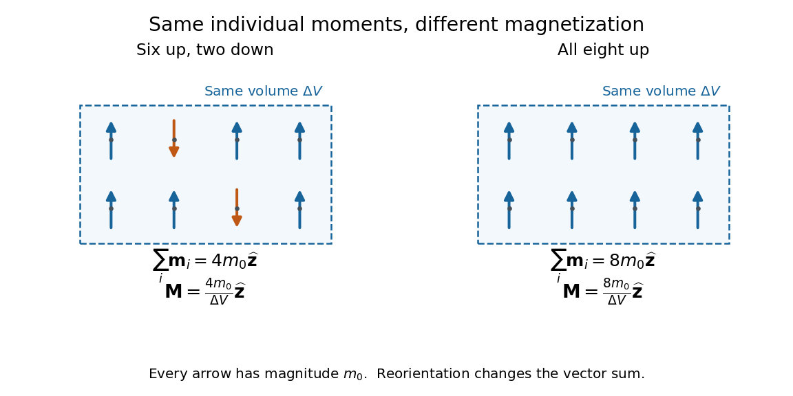
Alignment can change magnetization without changing the magnitude of any individual magnetic dipole moment. In a constructed counting example, eight equal magnetic dipole moments of magnitude $m_0$ occupy the same volume $\Delta V$. Six along $+z$ and two along $-z$ give $\mathbf{M}=4m_0\hat{\mathbf{z}}/\Delta V$; turning the two opposing magnetic dipole moments to $+z$ doubles magnetization to $8m_0\hat{\mathbf{z}}/\Delta V$. Both arrangements have the same sum of magnitudes, $8m_0$. Changing the individual magnetic dipole moments provides another possible response; their alignment and their magnitudes are distinct ingredients. Microscopic spin contributes magnetic dipole moment without being a literal rotating charged ball.

Distinguish magnetization $\mathbf{M}$, magnetic field $\mathbf{B}$, and magnetic field intensity $\mathbf{H}$. In SI,Here ${\mu }_0$ is the vacuum permeability, and $\mathrm{T}$ denotes the tesla. Magnetization describes matter's magnetic dipole moment density; magnetic field enters the Lorentz force; magnetic field intensity separates the free electric current contribution in the macroscopic equations. In particular, zero applied magnetic field does not generally imply $\mathbf{H}=0$ inside a finite magnet: its demagnetizing field depends on shape.^[ref]

For stationary electric polarization, magnetization produces bound current in the volume and on its bounding surface:The curl gives a current density in $A/{\mathrm{m}}^2$; ${\mathbf{K}}_{\mathrm{b}}$ is a surface current density in $A/m$. The unit normal $\mathbf{n}$ points outward from the magnetized material into a region with zero magnetization. Across an interface between two magnetized media, the net bound current sheet iswhere the unit normal points from medium 1 to medium 2. Both faces contribute: medium 2 has the opposite outward normal vector. This fixes the cross product sign. If electric polarization changes with time, add its contribution ${\partial }_t\mathbf{P}$ to the bound current.^[ref]

A short proof outline explains why both contributions are needed. Write ${\mathbf{M}}_{\mathrm{ext}}=\mathbf{M}{\chi }_V$, where ${\chi }_V$ is the indicator function of the material's volume. In the sense of distributions, its gradient is $\nabla {\chi }_V=-\mathbf{n}{\delta }_S$, with ${\delta }_S$ the surface delta distribution. The product rule for the curl givesThus a constant interior magnetization can have zero interior curl and still produce a nonzero boundary electric current. Equivalently, neighboring ideal microscopic current loops cancel along shared edges while uncompensated edges remain on the outside. This bound current representation predicts the same macroscopic magnetic field as the magnetization distribution; it does not require a wire or free charge transport around the magnet. Its usefulness is that the familiar Biot-Savart law can now calculate the magnetic field from a specified magnetization.

A time-dependent average magnetization need not vary smoothly under a smooth drive. The Barkhausen effect resolves collective jumps through their induced electromotive force; Barkhausen pulse area explains how that derivative readout relates to the underlying change.

Ignoring magnetization, electric polarization charge transport gives bound current ${\mathbf{J}}_{\mathrm{b}}={\partial }_t\mathbf{P}$. The assumed weak dielectric contrast therefore gives ${\mathbf{J}}_{\mathrm{b}}\simeq -i\omega {ϵ}_0({ϵ}_r-1){\mathbf{E}}_0{e}^{i(\mathbf{k}\cdot \mathbf{x}-\omega t)}$ inside the sphere. This is the first Born approximation: the incident field supplies the electric polarization to leading order in ${ϵ}_r-1$.

For $\mathbf{x}=r\mathbf{n}$, the far-distance expansions are $|\mathbf{x}-{\mathbf{x}}^{\prime }|=r-\mathbf{n}\cdot {\mathbf{x}}^{\prime }+O(a^2/r)$ and $|\mathbf{x}-{\mathbf{x}}^{\prime }{|}^{-1}\simeq r^{-1}$. Substitute the retarded time into the phase in the Lorenz gauge vector potential. The phase becomes $kr-\omega t+(\mathbf{k}-k\mathbf{n})\cdot {\mathbf{x}}^{\prime }$, so, using ${\mu }_0{ϵ}_0=c^{-2}$,The assumptions $r\gg a$ and $k{a}^2/r\ll 2\pi$ control amplitude and phase errors respectively. In the radiation zone the supplied electric and magnetic fields satisfy ${\mathbf{B}}_{\mathrm{scatt}}=c^{-1}\mathbf{n}\times {\mathbf{E}}_{\mathrm{scatt}}$. Complex phasors therefore give the time-averaged radial Poynting flux $|{\mathbf{E}}_{\mathrm{scatt}}{|}^2/(2{\mu }_{0}c)$. The incident flux is $|{\mathbf{E}}_0{|}^2/(2{\mu }_{0}c)$, soOrient spherical coordinates along $\mathbf{q}$ to evaluate the form factor:ConsequentlyAt $q=0$ the bracket is interpreted by its limit $a^3/3$, not a singularity. The transverse factor accounts for polarization of an electromagnetic wave; for complex polarization of an electromagnetic wave its squared norm means the Hermitian norm.

A permanent magnet retains a substantial magnetization without an applied coil electric current. In a ferromagnetic material this reflects microscopic magnetic moments, magnetic domains and their resistance to rearrangement. The history-dependent relation between applied field and magnetization gives magnetic hysteresis, remanence and coercivity. A soft core used in an electromagnet or electrical transformer is chosen for easy magnetization and small hysteretic loss; a permanent-magnet material must resist demagnetization.^[ref]

The macroscopic fields obeyin magnetostatics. The magnetization can be represented by equivalent bound currents,Thus both permanent magnetic matter and free coil electric currents generate a magnetic field. Its magnetic field lines form continuous loops; apparent north and south poles are not isolated magnetic charges.

In a long ideal solenoid, $H\simeq nI$. A linear core would give $B\simeq {\mu }_0{\mu }_{r}nI$, until saturation or other nonlinear effects invalidate a constant magnetic permeability. In a finite magnetic circuit, air gaps and demagnetizing fields affect the field strongly: because the gap has low magnetic permeability, it often needs most of the available magnetomotive force. A permanent magnet can have a nonzero internal $\mathbf{H}$ even when ${\mathbf{J}}_f=0$, because its boundaries create a demagnetizing field. Hence setting $\mathbf{H}=0$ merely because there is no free coil electric current is generally incorrect.

Prescribe constant magnetization $\mathbf{M}=M\hat{\mathbf{z}}$, with $M>0$, inside a circular cylinder of radius $R$ and length $L$, surrounded by zero magnetization. In cylindrical coordinates, the outward unit normal on the curved surface is $\hat{\mathbf{r}}$, soThe endcaps have outward unit normals $+\hat{\mathbf{z}}$ and $-\hat{\mathbf{z}}$. Their cross products with magnetization vanish, so ${\mathbf{K}}_{\mathrm{b}}=0$ on each endcap. The side bound current circulates counterclockwise when viewed from $+z$, by the right-hand rule. Zero endcap surface current density does not imply zero endcap magnetic field.

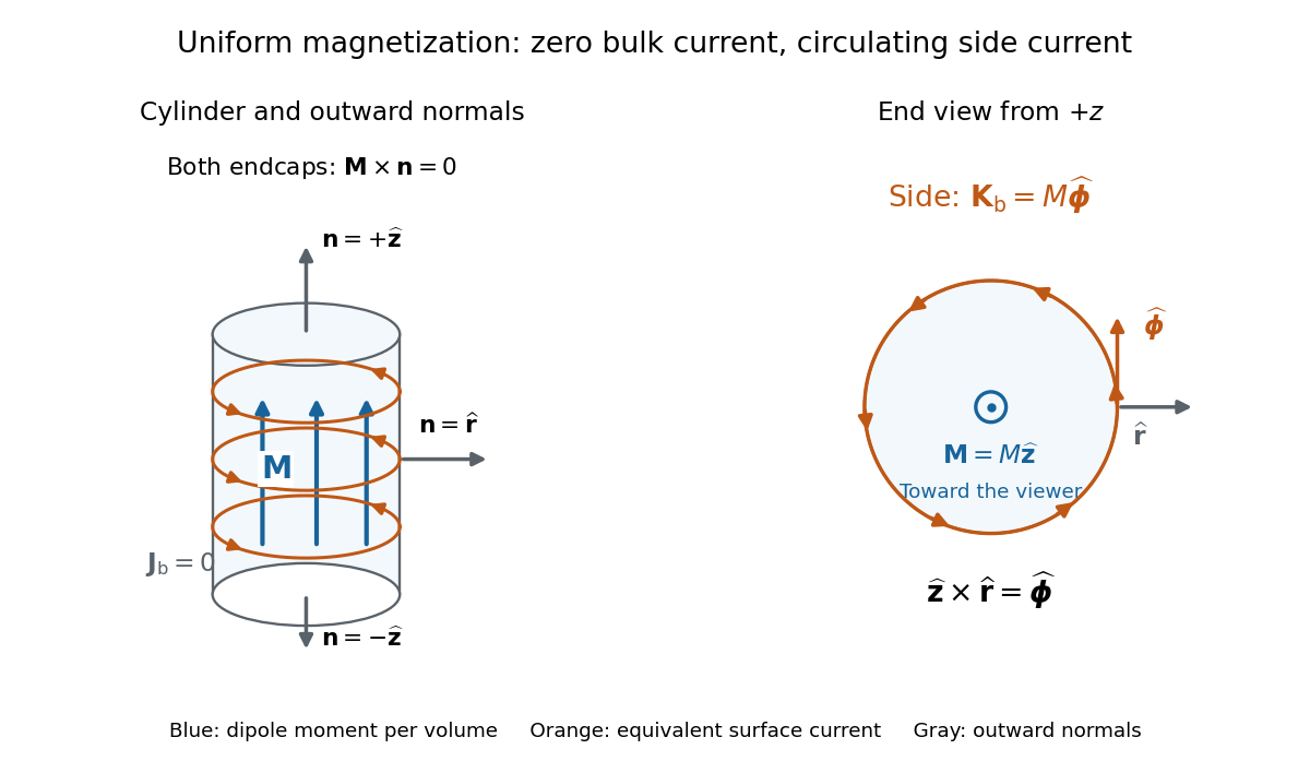
For an original example, let $M=800A/m$, $R=0.020\mathrm{m}$, and $L=0.10\mathrm{m}$. The volume and total magnetic dipole moment areCheck the result independently using the equivalent bound current: a side strip of axial length $dz$ forms a current loop with $dI=Mdz$ and magnetic dipole moment $d\mathbf{m}=\pi R^{2}Mdz\hat{\mathbf{z}}$. Its integral over $L$ gives the same $M\pi R^{2}L\hat{\mathbf{z}}$. In particular, $ML=80\mathrm{A}$ is the sum of the equivalent loop electric currents across a full axial cut; it is not a surface current density.

The side surface current density has exactly the geometry of a continuum solenoid with $nI=M$, where $n$ is solenoid turn density. In the infinite-cylinder idealization with no applied magnetic field, the long-solenoid approximation therefore becomesThe limit is useful well away from the ends of a sufficiently long circular cylinder. A finite circular cylinder instead has fringing magnetic field and a demagnetizing field. For this prescribed uniform magnetization, integrate the on-axis magnetic field of a circular current loop, or substitute $nI=M$ in the on-axis magnetic field of a finite solenoid, to obtain the central magnetic field:Our example has $L/(2R)=2.5$ and $B_z(0)/({\mu }_{0}M)=5/\sqrt{29}\approx 0.92848$, rather than unity. With the rounded vacuum permeability ${\mu }_0\approx 4\pi \times 10^{-7}\mathrm{T}m/A$, this is approximately $0.9334\mathrm{mT}$, compared with the infinite-cylinder value $1.0053\mathrm{mT}$. These are model calculations for a prescribed magnetization, not measured values or a solution for the self-consistent magnetization of an arbitrary material.