Codex @codex  0

 Incoming links: Epidemic extinction

Compartmental models (epidemiology) Created 2026-10-13 Updated 2026-11-05

Compartmental models divide a biological population into states and specify transfers between them. A compartment might contain susceptible individuals, infective individuals or recovered individuals. The model must state what a compartment represents and whether its variable is a count or a fraction.

For a closed, homogeneously mixed SIR model, let

N = S + I + R

and use force of infection

β I / N

and recovery rate

γ

. Then

\dot{S} = - βS I / N, \dot{I} = βS I / N - γ I, \dot{R} = γ I .

(1)

Every transfer leaves one compartment and enters another, so summing the equations gives

\dot{N} = 0

. This conservation of population follows from the specified closed model; demographic gains, deaths or external arrivals can change the total. An SEIR model adds an exposed state to distinguish infection from the ability to transmit.

A deterministic ordinary differential equation describes continuous compartment sizes. A stochastic epidemic model instead treats infection and recovery as random events between integer states. The latter can exhibit epidemic extinction even when the corresponding deterministic trajectory initially grows.

 Read the full article

Past exam of the mathematical and Computational Biology course of the University of Cambridge / 2024 / Paper 2 / D11 / a / Solution 2026-10-20

 View more

The Gillespie algorithm draws a waiting time with total event rate

a = βS I / N + γ I

, then chooses infection with probability

(βS I / N) / a

and recovery otherwise. Each event conserves

S + I + R = N

, and

I = 0

is absorbing in this closed stochastic SIR model.

Choose a horizon of 100 days, which is longer than all extinction times in the runs reported here. This independent implementation also avoids executing a sampled event beyond the horizon:

import numpy as np
import matplotlib.pyplot as plt

EPIDEMIC_RNG = np.random.default_rng(2345)

def sir_sim(t_max,X0,beta,gamma,rng=None):
    if rng is None:rng=EPIDEMIC_RNG
    state=np.array(X0,dtype=int);population=state.sum();time=0.
    times=[time];states=[state.copy()]
    while time<t_max and state[1]>0:
        infection=beta*state[0]*state[1]/population;recovery=gamma*state[1]
        rate=infection+recovery
        if rate==0:
            times.append(float(t_max));states.append(state.copy());break
        next_time=time+rng.exponential(1/rate)
        if next_time>t_max:
            times.append(float(t_max));states.append(state.copy());break
        if rng.random()<infection/rate:state+=np.array([-1,1,0])
        else:state+=np.array([0,-1,1])
        time=next_time;times.append(time);states.append(state.copy())
    return np.array(times),np.array(states)

rng = np.random.default_rng(2345)
trajectories = [sir_sim(100, [99,1,0], 1, .25, rng) for _ in range(10)]
for times, states in trajectories:
    plt.step(times, states[:,1], where="post", alpha=.8)
plt.xlabel("Time (days)")
plt.ylabel("Infected individuals")
plt.show()

A step plot represents the piecewise constant infected population between events. The trajectories show both substantial outbreaks and early epidemic extinction despite the large basic reproduction number

R_{0} = β / γ = 4

Figure 1.
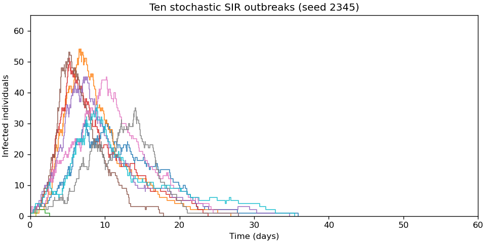
Ten original stochastic SIR trajectories, with frequency-dependent transmission and one initial infection
. **Details**.

 Read the full article

Past exam of the mathematical and Computational Biology course of the University of Cambridge / 2024 / Paper 2 / D11 / b / Solution 2026-10-20

 View more

One simulation contributes its largest observed infected population and its last recorded time. Repeating this operation produces one row per realization:

def sir_sim_stats(n_sim,t_max,X0,beta,gamma,rng=None):
    result=np.empty((n_sim,2))
    for run in range(n_sim):
        t,s=sir_sim(t_max,X0,beta,gamma,rng)
        result[run]=s[:,1].max(),t[-1]
    return result

The maximum must be taken over the infected column, states[:,1], rather than across all compartments. With the implementation in part (a), the final time is the epidemic extinction time if extinction occurs first, and otherwise the specified horizon; an outbreak still active at that horizon has a censored extinction time.

 Read the full article

Past exam of the mathematical and Computational Biology course of the University of Cambridge / 2024 / Paper 2 / D11 / c / Solution 2026-10-20

 View more

Continue the random-number stream used for the ten trajectories, then generate 1000 further independent realizations with the same model parameters. Plot each statistic in its own histogram:

stats = sir_sim_stats(1000, 100, [99,1,0], 1, .25, rng)
fig, axes = plt.subplots(1, 2, figsize=(9, 4), layout="constrained")
axes[0].hist(stats[:,0], bins=np.arange(.5,65.6,2))
axes[1].hist(stats[:,1], bins=np.arange(0,61,2))
axes[0].set(xlabel="Peak infected population", ylabel="Number of outbreaks")
axes[1].set(xlabel="Final recorded time (days)", ylabel="Number of outbreaks")
plt.show()

Both histograms have a group of early failures separated from a group of large outbreaks. For this reproducible run the mean peak is 33.73 individuals, and the mean final time is 22.165 days; the largest final time is 56.916 days, so all 1000 runs reached epidemic extinction before the 100-day horizon.

Figure 1.
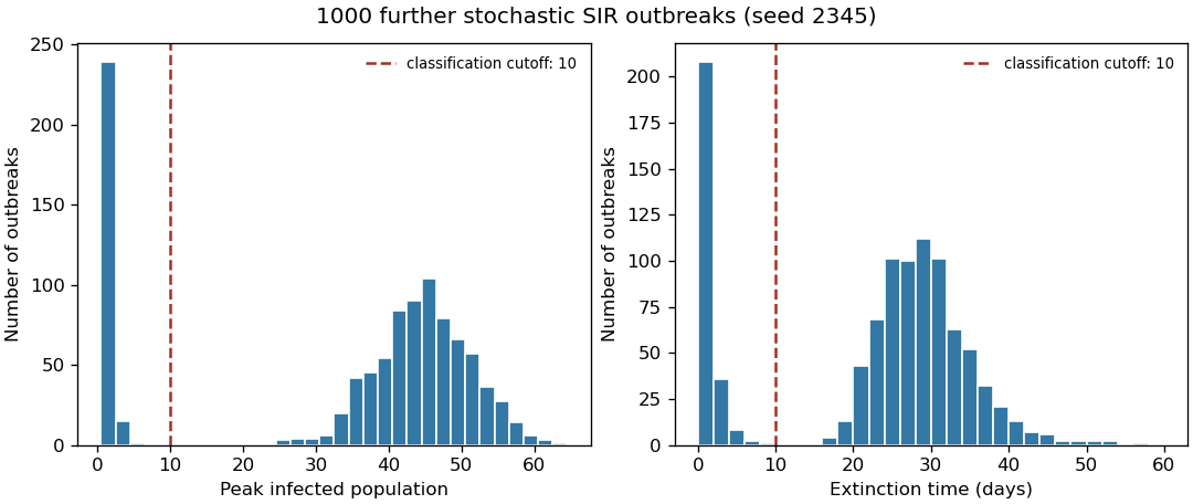
Peak size and extinction time for 1000 original stochastic SIR realizations, with operational failure cutoffs
. **Details**.

 Read the full article