A compartmental model divides a conserved population into states and uses differential equations for transition rates.
A compartment is one of the state categories in a compartmental model. Its state variable measures the number or amount in that category, and transfer terms record exchanges between compartments.
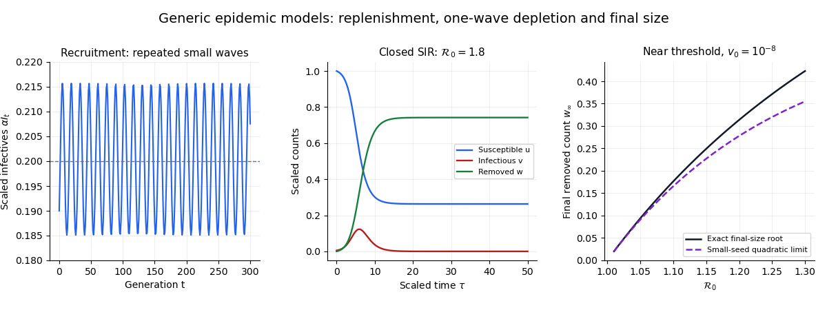
This generation-based compartmental model replenishes the susceptible compartment by per step and transfers individuals into the next infectious generation. Members of the current infectious compartment leave it after one step. In scaled variables , , , the update is , .
Its only fixed point is . There is no finite disease-free fixed point, since susceptible recruitment continues when . The Jacobian matrix at the fixed point is , with determinant one and trace . For , its two distinct eigenvalues have modulus one, so the linearized iterates are bounded and oscillatory. At , the repeated eigenvalue has a nontrivial Jordan block, making generic linearized iterates grow linearly. For , one eigenvalue has modulus greater than one.
Thus gives neutral linear stability, not asymptotic stability. Unit-modulus multipliers do not determine nonlinear stability. Recruitment can restore susceptibility above after a wave, allowing repeated infection growth; a closed SIR model without replenishment has a different susceptible balance.
An SIS model returns recovered hosts directly to susceptibility, so immunity does not accumulate. For homogeneous frequency-dependent transmission, a positive endemic state exists at when . This epidemiological model is distinct from the galaxy-dynamics abbreviation SIS for a singular isothermal sphere.
For high-risk group fraction , fixed total contact rates and reciprocal cross-group contacts, let . The displayed SIS model describes within-group infectious fractions. In fractions the transmission matrix is ; in infected-person counts it is . A common recovery rate gives basic reproduction number . The mean population susceptible fraction does not generally equal its reciprocal.
For fixed , let . The rare high-risk group's SIS model has , whereas low-risk infection is . Substitution into both equilibrium equations proves these coefficients. The leading basic reproduction number is with correction , while global susceptibility tends to one. These expressions explain why an endemic core can coexist with a large susceptible majority; they are nonuniform when a group is near its own threshold.
For , a positive endemic equilibrium requires and gives susceptible fraction . Below threshold the disease-free susceptible fraction is one. The reciprocal relation is a property of this homogeneous scalar SIS model, not a universal identity for heterogeneous populations.
For two otherwise symmetric SIS models with recovery rate , primary transmission and secondary susceptibility multiplier , split hosts into uninfected, singly infected and doubly infected classes. The displayed conditions give stable disease-free and joint endemic states, with an intermediate saddle: a strong Allee effect. The endemic susceptible fraction solves . The smaller root is the stable high-prevalence state. Coinfected hosts recover each infection independently, so recovery from coinfection leads to a single-infection class rather than directly to complete susceptibility.
If every transition transfers individuals between compartments without births, deaths, immigration, or emigration, the sum of all compartment sizes is constant.
Disease prevalence is the proportion of a population that is infected at a specified time. In a susceptible-infective model with total population , it is .
The SI model divides a closed population into susceptible and permanently infectious compartments. Under frequency-dependent homogeneous mixing,and conservation of population gives .
The stochastic SI model with susceptible fraction , initial limit , and total infection rate has deterministic limitThe Poisson time-change representation of a Markov chain writes as its integrated drift minus a centered Poisson error. On its clock is at most . The Poisson maximal concentration bound makes every fixed error tolerance have summable probabilities in , so the Borel-Cantelli lemma gives uniform error decay almost surely. The Gronwall inequality transfers that decay to , because the drift is Lipschitz continuous. The assertion is for fixed finite intervals and does not claim approximation over times growing with .
The plant-disease modelhas total population and disease prevalence satisfyingThus infection does not alter total-population growth. The invasion threshold at the carrying capacity is .
Removing susceptible and infected plants at the same per-capita rate changes the reduced equations toFor , the surviving population has carrying capacity , and infection invades precisely when .
The SEIR model divides a population into susceptible, exposed, infectious, and recovered compartments.
The force of infection is the instantaneous infection hazard experienced by a susceptible individual. Under homogeneous frequency-dependent mixing it is .
For a closed homogeneous epidemic, integrating relates the ultimately susceptible population to cumulative infections through an exponential equation.
The relation constrains the final outcome of compartmental models rather than describing their whole time-dependent solution.
Normalize the closed SIR model by its initial susceptible count, writing , , and . Then , and the SIR susceptible-recovered identity becomes . HenceThe positive root of the quadratic approximation isThe displayed small-seed formula requires , and . In particular, a regime is with a much smaller positive seed. Setting the seed exactly to zero produces the disease-free trajectory instead of an outbreak.

Homogeneous mixing assumes that contacts sample the whole modelled population without differences between groups or locations. In the SIR model, the chance that a sampled contact belongs to the infectious compartment is . This assumption makes a frequency-dependent transmission rule depend on the overall infectious compartment rather than a graph of individual contacts. Structured contacts require a different mathematical model, such as a discrete SIR epidemic on a graph.
For frequency-dependent transmission with homogeneous mixing, each member of the susceptible compartment experiences force of infection . Consequently the total flow into the infectious compartment is people per unit time. The constant combines the contact frequency and the chance that a relevant contact causes infection, and has units of inverse time. Holding the infectious compartment's fraction fixed holds each person's force of infection fixed when changes. An unnormalized mass-action infection convention instead writes the total flow as , where has units of inverse person-time; these two coefficients must not be confused.
The SIR model is a mathematical model of an epidemic that follows three groups: a susceptible compartment whose members can acquire infection, an infectious compartment whose members can pass it on, and a removed compartment whose members neither acquire nor pass on infection. The letters stand for susceptible, infectious and recovered or removed. Here we study the simplest closed, constant-parameter version, with homogeneous mixing and no births, deaths, migration or waning immunity. A person who leaves the infectious compartment never returns to the susceptible compartment in this version.[ref]
https://ocw.mit.edu/courses/1-022-introduction-to-network-models-fall-2018/fe3c864fd7d2d45ed7fe65e601d9c69e_MIT1_022F18_lec20.pdf. Amir Ajorlou, MIT Lecture 20: Epidemics, slides 18 and 24
The appeal of the SIR model is that one can explain a rise and fall in the infectious compartment without changing anyone's behavior: fewer opportunities for new infection eventually reverse the growth. The SIR first integral even determines the SIR infection peak without computing its time. These are useful deductions from explicit assumptions. The stipulated numbers below illustrate the mathematical model; they are neither estimates for an actual disease nor a forecast or medical advice.
Kermack and McKendrick's 1927 paper, "A contribution to the mathematical theory of epidemics", in Proceedings of the Royal Society A, is an early foundation for the SIR model. Its DOI is
10.1098/rspa.1927.0118, also recorded in the Royal Society's archive of contemporary referee reports.[ref]https://doi.org/10.1098/rspa.1927.0118. Kermack and McKendrick, original 1927 paper
[ref]https://catalogues.royalsociety.org/CalmView/Record.aspx?id=RR%2F35%2F131&src=CalmView.Catalog. Royal Society archive: contemporary referee report and publication record
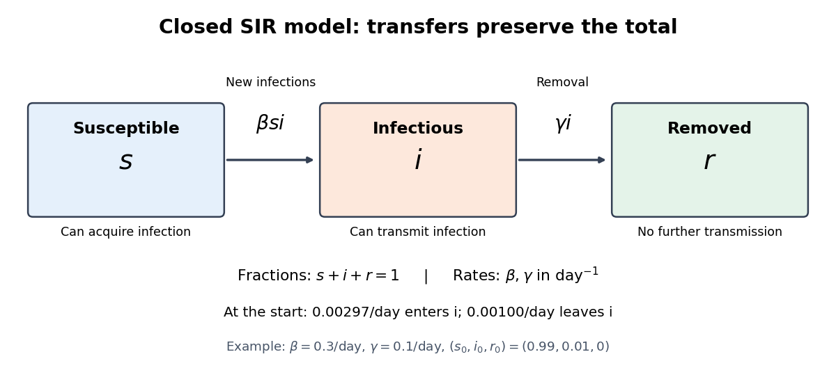
Transfers between the three compartments of the SIR model
. The SIR model equations transfer a fraction per day from the susceptible compartment to the infectious compartment, and a fraction per day from the infectious compartment to the removed compartment. Each arrow contributes a loss to one group and an equal gain to another, giving conservation of population. Details.
An infective individual is currently capable of transmitting the modeled infection. This is distinct from a susceptible individual and, when incubation is modeled, from an exposed individual not yet infectious.
In a compartmental epidemic model, a susceptible individual is one who can acquire the modeled infection. The susceptible compartment counts these individuals. An exposed but not yet infectious individual belongs to a separate latent class in an SEIR model; models that retain such individuals in a not-yet-infective compartment must state that bookkeeping convention explicitly.
A fatal-infection model with vaccination proportional to infective-susceptible encounters adds and . The total count including deaths is conserved. Integrating and gives and . The selected final root has , and deaths are . The model is a specified deterministic reaction scheme, not a general vaccination policy rule.
The susceptible compartment consists of people who can acquire infection. In the closed SIR model, is their count and their fraction of the fixed total . Membership expresses the assumptions of the mathematical model, rather than measuring the strength of an individual's immunity.
The infectious compartment consists of people currently able to transmit infection. In the closed SIR model, is their count and their fraction of the fixed total . The SIR model has no separate delay between acquiring infection and entering the infectious compartment; the SEIR model adds such a stage.
The removed compartment consists of people permanently excluded from both acquiring and passing on infection in the SIR model. Its count is and its fraction is . Removal can represent regained health with lasting immunity, or another permanent exclusion from acquiring or passing on infection; it need not mean being healthy again. Here there are no deaths. In a variant that counts deaths within , conservation of population would concern the original cohort, rather than the number currently alive.[ref]
For frequency-dependent transmission, the closed SIR model is a system of ordinary differential equations for the fractions :Here is the coefficient of frequency-dependent transmission, and is the recovery rate, interpreted more generally as the removal rate. Both have units of inverse time. With a constant recovery rate, the associated individual time in the infectious compartment has an exponential distribution with mean ; the SIR model does not require every person to spend exactly that long there. The fractions themselves have no units.[ref]
For counts , , , the same SIR model equations readThe factor keeps the same in both descriptions. Dropping it while keeping these units would fail dimensional analysis. Some existing SIR model variants use the unnormalized mass-action infection convention instead, including the SIR susceptible-recovered identity; their coefficient is in the notation used here.
Adding the SIR model equations gives , a short proof of conservation of population. Nonnegative starting fractions stay nonnegative: the outflow from either the susceptible compartment or the infectious compartment vanishes when that group is empty, while . Thus the susceptible compartment can only shrink and the removed compartment can only grow.
For a concrete initial value problem, stipulateAt the start, the flow into the infectious compartment is of the total per day, and the flow into the removed compartment is of the total per day. Hence per day. If , these correspond to model rates of and people per day, and net growth people per day. A rate need not be an integer count of events on any particular day.
For this SIR model, the basic reproduction number isIt describes one introduced member of the infectious compartment in an otherwise wholly susceptible compartment. The instantaneous reproduction number at the actual starting state is , obtained by freezing the current conditions and the current susceptible compartment's fraction. More generally it is in this SIR model. The basic reproduction number is a ratio of two rates, so it has no units; is a different quantity, the initial removed compartment's fraction.
While , its instantaneous relative growth isInitially this equals . Freezing gives the early exponential growth approximation with measured in days. It must fail as the susceptible compartment shrinks. An epidemic invasion threshold occurs at ; if , the deterministic SIR model stays at even above that threshold.
For , the SIR model equations have the first integral of an ordinary differential equationHere is the natural logarithm. A short proof outline is to use the chain rule and substitute the SIR model equations:The SIR first integral gives directly from , so it describes the curve in a phase portrait even before its time parametrization is known.
If and , the infectious compartment initially grows. The SIR model equations give its unique later maximum whenBefore this SIR infection peak, ; afterward it is negative because the susceptible compartment keeps shrinking. Substituting into the SIR first integral givesFor the stipulated initial value problem,Thus about of the modelled population belongs to the infectious compartment simultaneously at the SIR infection peak. This is a peak of the infectious compartment, not of incidence, whose flow is . If , the maximum is already at the start and the interior SIR infection peak formula does not apply.
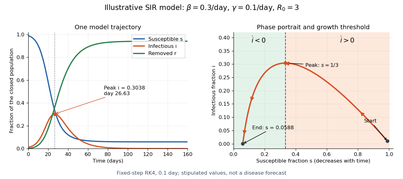

The numerical solution of a differential equation puts the SIR infection peak at about day with , agreeing with the SIR first integral to within . The accompanying generator checks nonnegative fractions and conservation of population without clipping or rescaling. For steps , and day, the largest differences between successive numerical trajectories at shared times are approximately and . Their ratio is , close to the factor expected when a fourth-order Runge-Kutta method's step is halved.
For the closed SIR model with , the infectious compartment's fraction approaches . One proof outline uses the bounded, increasing removed compartment's fraction: since , the total time-integrated is finite. The bounded derivative from the SIR model equations prevents indefinitely recurring spikes, so tends to zero.
For , the final size relation for an epidemic follows by dividing the SIR model equations for and while , giving . Integration then yieldsThis also follows from the SIR first integral and conservation of population. For the stipulated initial value problem, solveThe bisection method givesAbout of the original population remains in the susceptible compartment. The is the final removed compartment's fraction, including the initially in the infectious compartment. The newly acquired infection during the modelled period accounts for of the total population, not . Dividing by instead gives the proportion of initially susceptible compartment members who acquire infection; its denominator must be stated.
At the SIR infection peak, the flow into the infectious compartment only balances its outflow; it does not stop. Further infection explains why the final susceptible compartment's fraction is well below . Also for and finite : the closed SIR model does not require everybody to acquire infection before its infectious compartment empties in the long-time limit.
Here and weight susceptibility and infectiousness of a farm with animals, with size distribution and recovery rate . The rank-one next-generation matrix has reproduction number . Susceptibility proportional to size preferentially depletes large susceptible farms. Infectivity heterogeneity alone leaves an exactly homogeneous aggregate SIR trajectory for representative initial infections. When both weights equal size, the second rather than first size moment governs invasion.
In this discrete-time SIR model, each infected vertex is infectious for one step, can infect each susceptible neighbour with probability , and is then permanently removed. The adjacency matrix of a graph describes the possible transmissions. If the initial removed set is empty, eventual removal and ever becoming infected are the same event.
The conditional union bound gives in a discrete SIR epidemic on a graph. Iteration bounds the infection vector at step by . Each vertex is infected at most once, so summing the probabilities in time gives the displayed bound. Powers of the adjacency matrix of a graph count walks, which can overcount impossible reinfections without invalidating the upper bound. Initially removed individuals must be counted separately when bounding all eventual removals.
When , summing the adjacency-matrix bound for a discrete SIR epidemic gives the displayed Neumann series bound on the expected total infected count . For an undirected graph, the adjacency matrix of a graph is a symmetric matrix, so its Euclidean operator norm equals its spectral radius. The Cauchy-Schwarz inequality then yields for initially infected vertices.
The displayed condition and the resolvent bound for a discrete SIR epidemic imply . The Markov inequality then makes in probability. A sufficient special case is a sublinear initial infected count with a fixed positive gap . The inequality at each finite population size alone does not control a shrinking gap or an initially macroscopic outbreak.
The deterministic SIR model with initial susceptible count grows initially exactly when . Its basic reproduction number is under unnormalized mass-action infection. If that ratio is at most one, decreasing prevents later infectious growth.
For the closed deterministic SIR model with , , infection rate and recovery rate , division of the two flow equations gives . Population conservation then expresses in terms of .
The stochastic SIR model is a continuous-time Markov chain with infection jump at rate and recovery jump at rate . The state space consists of nonnegative integer compartment counts with conserved total population.
An epidemic reaches an absorbing state when no infected individuals remain and there is no external source of infection. Extinction time differs from a simulation horizon at which infected individuals are still present.
With one initial infectious individual, two events require an infection as the first event. If it occurs at time , its density is and the next total event rate is . Integrating this density times the chance of another event before a fixed horizon gives the two-event probability.
A chain-binomial epidemic model uses discrete time, with conditionally independent binomial distributions for infection and recovery counts given the current compartments. It requires valid probability parameters; replacing by is a small-step approximation.
Under mass action, random pairwise encounters between populations of sizes and occur at a rate proportional to .
A spatial SIR-type model combines compartment transitions with diffusion in the compartments whose members move appreciably.
For a pulse in which only infectives diffuse, the travelling-wave equations imply and . Integrating total biological population balance with vanishing infective derivative at both infinities gives the displayed final-size relation. Its nontrivial root requires . Thus deaths are exactly , while live density behind the wave is . The root is independent of in this particular pulse model.
Mass-action transmission at unit nondimensional rate transfers population from susceptible to infected compartments at rate .
A Laplacian term in the infected-population equation models unbiased random migration of infective individuals.
A disease-free equilibrium is an equilibrium of an epidemic model at which every infected compartment is zero.
An endemic equilibrium is an equilibrium at which infection persists, so at least one infected compartment is positive.
The equationscombine mass-action infection with an exponential density-dependent birth model. Susceptibles reproduce at per-capita rate , while infectives have no reproductive term and die at total per-capita rate .
When the disease-free equilibrium is unstable, the positive equilibrium satisfiesIts Jacobian has negative trace and positive determinant, so the equilibrium is locally asymptotically stable.
The basic reproduction number is the expected number of secondary infections caused by one infective in an otherwise susceptible population.
The entry is the expected number of newly infected type- individuals produced by a newly infected type- individual while the population is disease-free. In a compartmental linearization, describes new-infection production and transitions and removal. Provided the infection-lifetime subsystem is transient, its integrated occupation matrix is , yielding . The basic reproduction number is its spectral radius. This construction is described in the original next-generation-matrix derivation.
For a heterogeneous SIS model with common recovery rate and a positive endemic equilibrium , force balance gives . When the transmission matrix is irreducible and nonnegative, the positive equilibrium vector and the Perron–Frobenius theorem imply the displayed spectral radius identity. It replaces the homogeneous scalar relation : different recipient types generally have different susceptible fractions.
With susceptible, infective, and immune populations , equal per-capita birth and death rate , mass-action transmission coefficient , and recovery rate , the equations areThe conserved population is , and the threshold population is .
When , the positive equilibrium isOn the invariant plane , the Jacobian at this equilibrium has negative trace and positive determinant , so both eigenvalues have negative real part and the equilibrium is locally asymptotically stable.
For susceptible, infective, and recovered populations , mass-action infection coefficient , recovery rate , and immunity-loss rate , the SIRS equations areThey conserve and have basic reproduction number .
In a closed population of size , a frequency-dependent SIRS epidemic has the displayed transitions at rates , , and . The exponential distribution of infectious lifetimes and the constant immunity-loss hazard make the compartment counts a continuous-time Markov chain. Each jump preserves .
For convergent initial proportions, the scaled SIRS Markov chain converges uniformly in probability on each fixed finite interval to the solution of these equations. The Poisson time-change representation of a Markov chain writes it as its integrated drift plus centered Poisson errors. Bounded rates, Poisson concentration and the Gronwall inequality control the error. This finite-time limit does not by itself justify an approximation over time intervals growing with the population size.
When and , the positive equilibrium isWriting , the reduced Jacobian has characteristic polynomialBoth roots have negative real part. Its discriminant is negative for sufficiently small and positive for sufficiently large , giving respectively a stable focus and a stable node.
Articles by others on the same topic
There are currently no matching articles.