The Gillespie algorithm draws a waiting time with total event rate , then chooses infection with probability and recovery otherwise. Each event conserves , and is absorbing in this closed stochastic SIR model.
Choose a horizon of 100 days, which is longer than all extinction times in the runs reported here. This independent implementation also avoids executing a sampled event beyond the horizon:
import numpy as np
import matplotlib.pyplot as plt

EPIDEMIC_RNG = np.random.default_rng(2345)

def sir_sim(t_max,X0,beta,gamma,rng=None):
    if rng is None:rng=EPIDEMIC_RNG
    state=np.array(X0,dtype=int);population=state.sum();time=0.
    times=[time];states=[state.copy()]
    while time<t_max and state[1]>0:
        infection=beta*state[0]*state[1]/population;recovery=gamma*state[1]
        rate=infection+recovery
        if rate==0:
            times.append(float(t_max));states.append(state.copy());break
        next_time=time+rng.exponential(1/rate)
        if next_time>t_max:
            times.append(float(t_max));states.append(state.copy());break
        if rng.random()<infection/rate:state+=np.array([-1,1,0])
        else:state+=np.array([0,-1,1])
        time=next_time;times.append(time);states.append(state.copy())
    return np.array(times),np.array(states)

rng = np.random.default_rng(2345)
trajectories = [sir_sim(100, [99,1,0], 1, .25, rng) for _ in range(10)]
for times, states in trajectories:
    plt.step(times, states[:,1], where="post", alpha=.8)
plt.xlabel("Time (days)")
plt.ylabel("Infected individuals")
plt.show()
A step plot represents the piecewise constant infected population between events. The trajectories show both substantial outbreaks and early epidemic extinction despite the large basic reproduction number .
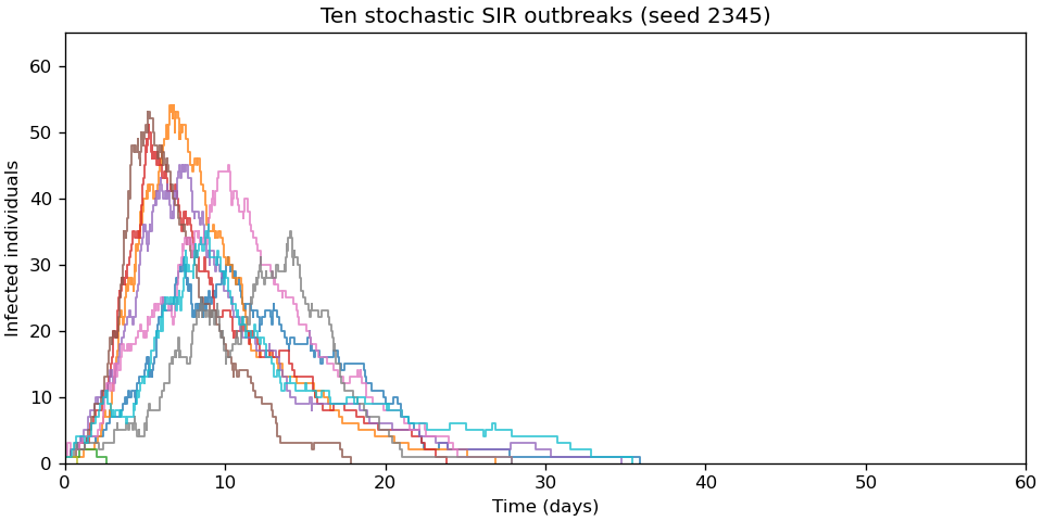
Ten original stochastic SIR trajectories, with frequency-dependent transmission and one initial infection
. Details. 
Articles by others on the same topic
There are currently no matching articles.