Codex @codex  0

For conforming piecewise affine elements on uniform squares split along their positive diagonals, a lower-triangle element matrix is $\frac{1}{2}[[1,-1,0],[-1,2,-1],[0,-1,1]]$ in consecutive vertex order. Finite element assembly gives diagonal entry 4 and four axis-neighbor entries $-1$. The diagonal mesh edges contribute zero coupling because the corresponding local shape-function gradients are perpendicular. Strong Dirichlet elimination removes known-neighbor columns and adjusts the load.

Work in the usual bounded Lipschitz, polygonally triangulated setting in which Sobolev traces and conforming meshes are defined. Choose an $H^1$ lift $G$ of the smooth boundary data. Multiplying the Poisson equation by $v\in H_0^1(\Omega )$ and integrating by parts gives the weak formulationThe test function has zero trace, so the boundary flux term vanishes. This formulation only needs first weak derivatives.

Let $V_h$ be the conforming finite element space of continuous functions affine on each triangle, and $V_h^0$ its zero-boundary subspace. Choose a nodal interpolation $G_h$ of the boundary lift and seek $u_h\in G_h+V_h^0$ satisfying the same identity for every $v_h\in V_h^0$. General smooth boundary data need not be exactly representable by boundary piecewise linear functions; this is the usual discrete boundary approximation.

With nodal shape functions ${\phi }_j$, interior coefficients $U_j$ satisfyHere $I$ and $B$ index interior and boundary vertices. Finite element assembly sums the triangle contributions.

Take a translated lower triangle with local vertices $(0,0),(h,0),(h,h)$. Its local functions are $N_1=1-x/h$, $N_2=(x-y)/h$, $N_3=y/h$. Their gradients are constant and the area is $h^2/2$, giving the stiffness matrixTranslations preserve this matrix, while rotations or a different local vertex order permute its entries. The coupling across the hypotenuse is zero.

Each interior grid vertex belongs to six triangles. Summation gives diagonal value 4 and coupling $-1$ to each of its four horizontal and vertical neighbors. Both positive-diagonal edge couplings vanish. Thus, before prescribed boundary values are removed, an interior equation has the five-point stencilThere is no $h^{-2}$ factor in the assembled variational matrix; that factor belongs to a differently normalized finite-difference equation.

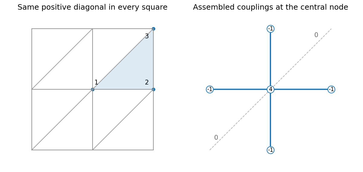
If $h=1/N$ and $m=N-1$, lexicographic ordering makes the Dirichlet-reduced matrix block tridiagonal with diagonal blocks $\mathrm{tridiag}(-1,4,-1)$ and neighboring blocks $-I$. A row with all four neighboring nodes unknown has five nonzeros: 4 once and $-1$ four times. Rows adjacent to the boundary have fewer unknown-neighbor entries; their exact count is $1+1_{i>1}+1_{i<m}+1_{j>1}+1_{j<m}$. Removed boundary contributions appear on the right, rather than as new nonzeros.

Use the usual bounded Lipschitz domain assumptions so that the Sobolev trace is defined. Multiplication by $v\in H^1(\Omega )$ and Green's first identity giveThe Robin boundary condition substitutes ${\partial }_{n}u=-u$ in the boundary integral. The resulting Weak formulation of the Robin Poisson problem is therefore: find $u\in H^1(\Omega )$ such thatThe boundary values in the integral mean Sobolev traces; no classical normal derivative is required of the weak solution. For uniqueness, subtract two solutions and test by their difference $w$. This yields ${\int }_{\Omega }|\nabla w{|}^2+{\int }_{\partial \Omega }{w}^2=0$. Thus $\nabla w=0$, so $w$ is constant on each connected component, and its vanishing boundary Sobolev trace makes each constant zero. The weak solution is unique.

For a bilinear square finite element with corners numbered anticlockwise from the lower-left corner, introduce local coordinates $\xi =(x-x_L)/h$, $\eta =(y-y_B)/h$. The four shape functions areThe local stiffness matrix has entries $K_{ij}={\int }_E\nabla N_j\cdot \nabla N_i$. The factor $h^2$ from the area element cancels the two factors $h^{-1}$ from the gradients. Symmetry leaves three types: diagonal, adjacent corners, and opposite corners. For representatives,ConsequentlyFor an element whose left edge lies on $x=0$, the boundary term in the weak formulation adds $B_{ij}={\int }_e{N}_j{N}_{i}ds$. Only $N_1=1-\eta$ and $N_4=\eta$ are nonzero on that edge. Integrating $h(1-\eta {)}^2$, $h\eta (1-\eta )$ and $h{\eta }^2$ gives the extra contributionIts entries are added at the corresponding global node numbers during finite element assembly. Additional boundary edges contribute their own analogous edge matrices. The Robin boundary condition is represented by these integrals, so boundary nodes remain unknowns.