Derivative ($\frac{df}{dx}$)

The derivative measures the instantaneous rate at which a function changes. For a real function $f$ defined near $a$, it exists when the difference quotient has a finite two-sided limit:The quotient is the slope of the straight line joining two nearby points of the graph. Its limit is the slope of the tangent line. Thus a derivative describes a local rate without choosing a particular finite measurement interval.

For $f(x)=x^2$, expanding the numerator givesAt $a=1$, the increments $h=1$, $1/2$ and $1/10$ give secant line slopes $3$, $2.5$ and $2.1$. The limit is $2$, and the tangent line is $y=1+2(x-1)$. The picture makes the limiting process visible.

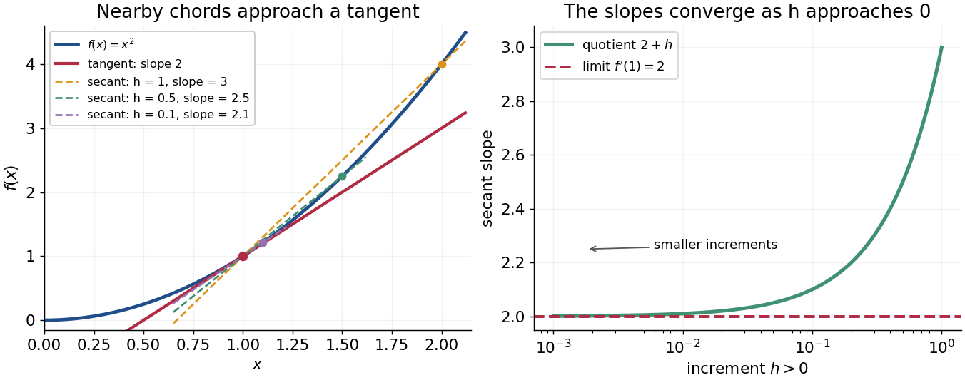
The same calculation shows why the derivative is useful for approximation:This is a local linear approximation. Near $a=1$, replacing $(1+h{)}^2$ by $1+2h$ makes the exact error $h^2$, smaller than the leading change when $h$ is small. A curved graph can therefore be studied locally using a straight line.

If the function records position against time, its derivative is velocity. If it records an objective function, its derivative tests local changes that matter in optimization; in several variables, the gradient collects these directional rates and guides gradient descent. The interpretation comes from the function and its units, rather than from a new rule for each application.

Existence matters. For the absolute value function $f(x)=|x|$, the one-sided derivatives at zero are $-1$ and $1$, so there is no single tangent line described by a finite derivative there. Nor does a zero derivative alone identify a maximum or minimum: $f(x)=x^3$ has $f^{\prime }(0)=0$ but keeps increasing through zero.

For a differentiable function, a local linear approximation replaces nearby values by its value plus its derivative times the input change. The error divided by that change tends to zero. It uses the first-order Taylor polynomial; the statement concerns a limit near the specified point, not a guaranteed approximation far from it.

The symmetric second derivative is the displayed limit when it exists. For a twice continuously differentiable function it equals the ordinary second derivative by Taylor expansion; the definition itself does not require ordinary differentiability. A continuous function with vanishing symmetric second derivative throughout an interval must be affine, by vanishing symmetric second derivative forces an affine function. For a twice-integrated Fourier series, sinc-squared weights express this quotient, connecting the operation to Riemann summation of a convergent trigonometric series.

For a continuous function with affine formulas $At+B$ to the left of $c$ and $A^{\prime }t+B^{\prime }$ to its right, the quotient $[F(c+h)-2F(c)+F(c-h)]/h$ equals $A^{\prime }-A$ for positive $h$. If it tends to zero, the slopes agree, and continuity at $c$ makes the intercepts agree as well. This detects slope jumps that ordinary pointwise derivatives away from the corner cannot detect.

For a continuous function with affine formulas $At+B$ to the left of $c$ and $A^{\prime }t+B^{\prime }$ to its right, the quotient $[F(c+h)-2F(c)+F(c-h)]/h$ equals $A^{\prime }-A$ for positive $h$. If it tends to zero, the slopes agree, and continuity at $c$ makes the intercepts agree as well. This detects slope jumps that ordinary pointwise derivatives away from the corner cannot detect.

If a continuous real function on an interval has the displayed limit zero at every interior point, it is affine. On any compact subinterval subtract its endpoint chord. If the difference were positive somewhere, adding $\epsilon (t-a)(t-b)$ for sufficiently small positive $\epsilon$ would retain a positive interior maximum. At a maximum every symmetric second difference is nonpositive, but its normalized limit would be $2\epsilon >0$. Thus the function lies below its chord; applying the same argument to its negative gives equality. Real and imaginary parts give the complex-valued version. Existence of ordinary second derivatives is unnecessary.

The right and left one-sided derivatives are the limits of the difference quotient restricted respectively to positive and negative increments:At an interior point, differentiability is equivalent to existence and equality of these two finite limits. For the absolute value function, $f_{+}^{\prime }(0)=1$ and $f_{-}^{\prime }(0)=-1$, so it is continuous at zero but not differentiable there.

The tangent line to a differentiable function at $a$ is its affine first-order approximation $f(a)+f^{\prime }(a)(x-a)$. For a differentiable concave function, it is an upper bound throughout a convex interval: the secant-slope inequality and passage to the derivative give $f(x)\le f(a)+f^{\prime }(a)(x-a)$. This upper bound constructs valid envelopes in adaptive rejection sampling.

Automatic differentiation evaluates derivatives of a computational graph using the chain rule. Reverse mode is backpropagation and is useful for reparameterization gradients through simulated trajectories.

Differentiation computes the derivative of a function. A difference quotient approximates a derivative using finite increments; its limit is the derivative when the function is differentiable.

The derivative of the first derivative. For a twice differentiable function, its sign governs local convexity and its magnitude controls the second-order Taylor remainder.

A difference quotient divides a finite change in a function by the corresponding change in its argument. Its limit, when it exists, is the derivative.

With ${\delta }_{h}f(x)=[f(x+h{e}_{\ell })-f(x)]/h$, a change of variables givesThe compact support of $f$ and its translates must remain inside the integration domain, or one must integrate over the whole space with convergent integrals. In particular ${\delta }_{-h}g(x)=[g(x)-g(x-h{e}_{\ell })]/h$: the denominator's sign matters. This is the difference quotient analogue of integration by parts.

A total derivative accounts for every dependence of a quantity on the variable of differentiation. For a differentiable function $F(t,x_1,\dots ,x_n)$ evaluated along differentiable coordinate functions $x_i(t)$, the multivariable chain rule givesAll the partial derivatives on the right are evaluated at $(t,x_1(t),\dots ,x_n(t))$. The first term captures explicit dependence on $t$; the remaining terms capture changes transmitted through the coordinates.

For example, take $F(t,x)=t{x}^2$ and $x(t)=t$. The partial derivative with respect to $t$, holding $x$ fixed, is $x^2$, whose value on the path is $t^2$. The total derivative is insteadAt $t=2$, the partial derivative is $4$ and the total derivative is $12$. The difference is the contribution from changing $x$.

If the composite function is continuously differentiable on $[a,b]$, the fundamental theorem of calculus givesThis is the sense in which an integrated total derivative contributes endpoint terms. The endpoint statement concerns the whole composite function along the path. ^[ref].

For an indeterminate quotient whose numerator and denominator both tend to zero or both diverge, suitable differentiability and denominator conditions allow its limit to be computed from the limit of the quotient of their derivatives.

The usual zero-over-zero L'Hopital rule requires the denominator's derivative to be nonzero throughout a sufficiently small deleted neighborhood. A limit taken only where that derivative is nonzero is insufficient. An explicit counterexample uses $x_n=2^{-n}$, $h_n=4^{-n}$, $S(u)=3u^2-2u^3$ and $q(u)=16u^2(1-u{)}^2$. On $[3x_n/4,x_n]$ put $g=h_n$ and $f=h_{n}q((x-3x_n/4)/(x_n/4))$. On $[x_n/2,3x_n/4]$ put $g=h_{n+1}+(h_n-h_{n+1})S((x-x_n/2)/(x_n/4))$ and $f=0$. Extend $g=1,f=0$ beyond one. Values and first derivatives agree at the joins, both functions tend to zero, and $g$ is positive. Where $g^{\prime }\ne 0$, it lies inside a transition interval and $f^{\prime }=0$. Thus $f^{\prime }/g^{\prime }$ has natural-domain limit zero, but $f/g$ equals zero at $x_n$ and one at $7x_n/8$, so has no limit.

Every derivative has the intermediate-value property, even when the derivative is discontinuous.

Let $m=(f(b)-f(a))/(b-a)$ for a function differentiable on a neighborhood of $[a,b]$. If $m=k$, use the whole interval. If $m>k$, the continuous extension of $(f(x)-f(a))/(x-a)$ takes values $f^{\prime }(a)$ and $m$ at the endpoints, so the intermediate value theorem supplies a secant of slope $k$ starting at $a$. If $m<k$, use the continuous extension of $(f(b)-f(x))/(b-x)$ and obtain a secant ending at $b$. The mean value theorem then produces an interior derivative equal to $k$, without requiring a continuous derivative.

If $f$ and $g$ are differentiable at $a$, then

For a continuous function $f:\mathbb{R}\to \mathbb{R}$, $g(t)=t^{2}f(t)$ is differentiable at zero with $g^{\prime }(0)=0$, because $[g(h)-g(0)]/h=hf(h)\to 0$. At any nonzero point $x$, $g$ is differentiable exactly when $f$ is: one direction uses the product rule, and the converse applies it to $f(t)=t^{-2}g(t)$ near $x$.

The higher-order product rule is

At zero, $f(x)=x$ and $g(x)=1+|x|$ give a differentiable productwith derivative one, although $g$ is not differentiable.

If $f$ and $g$ are differentiable and $g\ne 0$, then

The chain rule calculates the derivative of a function composition by combining local rates. If the inner function $f$ is differentiable at $a$ and the outer function $g$ is differentiable at $f(a)$, thenThe evaluation point matters: the outer derivative is evaluated at the inner output $f(a)$, not at $a$. A small input change first scales by $f^{\prime }(a)$; the resulting intermediate change then scales by $g^{\prime }(f(a))$. In terms of linear approximations, composing those two local descriptions multiplies their scale factors. ^[ref].

For example, $h(x)=\sin (x^2)$ applies a quadratic function and then the sine. With $f(x)=x^2$ and $g(u)=\sin u$, the chain rule givesHere all angles are in radians. Near $x=1$, increasing the input by $\Delta x$ changes $x^2$ by about $2\Delta x$, and the sine changes by about $\cos 1$ times that intermediate change. For $\Delta x=0.01$, the linear approximation predicts an output increase of $0.0108060$; the exact increase is $\sin (1.0201)-\sin 1\approx 0.0106894$.

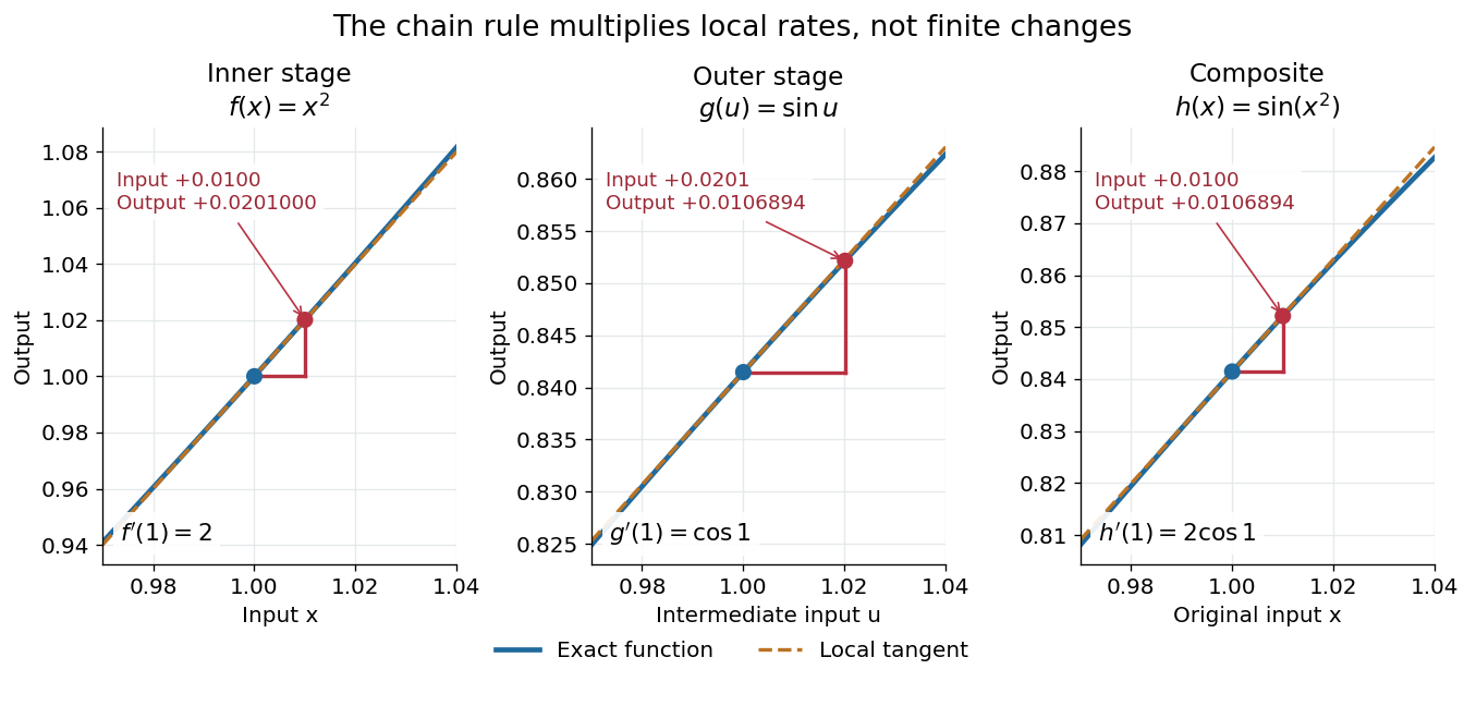
The same rule handles several nested stages. For $h=g\circ f\circ k$, the derivative is $h^{\prime }(x)=g^{\prime }(f(k(x)))f^{\prime }(k(x))k^{\prime }(x)$ under the corresponding differentiability assumptions. Writing each intermediate output prevents evaluating a derivative at the wrong stage. It also makes the chain rule useful for propagating sensitivities through a mathematical model, where one measured quantity influences another through several transformations.

For a quick proof idea, replace $f$ near $a$ by its linear approximation, then replace $g$ near $f(a)$ by its linear approximation. The composite leading term is their product; differentiability ensures the remaining error is smaller than the original input change. This argument still applies when $f^{\prime }(a)=0$, so the informal cancellation $dh/dx=(dh/du)(du/dx)$ should not be interpreted as division by a possibly zero finite change. The hypotheses are sufficient, but are not necessary for every composite to be differentiable, as the nondifferentiable inner function with a differentiable nondegenerate composite example shows.

A linear approximation replaces a differentiable function near a reference input by its value plus the first-order change supplied by its derivative. In one dimension, this is the tangent line $f(a)+f^{\prime }(a)(x-a)$. The chain rule combines such local approximations through function composition; it does not assert their equality to the original functions over a finite interval.

For differentiable maps $f:{\mathbb{R}}^n\to {\mathbb{R}}^m$ and $g:{\mathbb{R}}^m\to {\mathbb{R}}^r$, the multivariable chain rule multiplies their Jacobian matrices:The outer $r\times m$ matrix multiplies the inner $m\times n$ matrix, producing an $r\times n$ matrix. This order records that the inner linear map acts first. Componentwise, the matrix multiplication sums the contributions of all intermediate coordinates. Existence of separate partial derivatives alone is not the required differentiability hypothesis.

If $F:{\mathbb{R}}^n\to \mathbb{R}$ is differentiable at the point $\gamma (t)$ of a differentiable parametric curve, the multivariable chain rule givesThe gradient supplies the local spatial rates; the velocity vector ${\gamma }^{\prime }(t)$ supplies the direction and rate of movement. Their dot product is the change in the sampled scalar field per unit parameter. If the parameter is time, this is a rate per unit time; a directional derivative per unit distance instead uses a unit vector.

Take $F(x,y)=x^2+2y^2$ and the unit circle path $\gamma (t)=(\cos t,\sin t)$. Along the path,At $t=\pi /4$, the gradient is $(\sqrt{2},2\sqrt{2})$, the velocity vector is $(-1/\sqrt{2},1/\sqrt{2})$, and their dot product is $-1+2=1$. The sampled value is $3/2$ and increases at rate one, even though one coordinate is decreasing. This is why a moving observation must combine every coordinate's contribution.

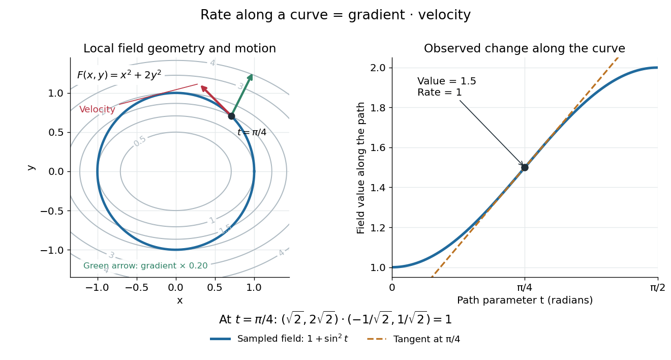
For a level curve, $F(\gamma (t))$ is constant, so the derivative along a curve is zero and its velocity vector is orthogonal to the gradient. Along other paths, the same formula combines a field's geometry with the observer's motion. ^[ref].

At zero, $f(x)=\sqrt[3]{x}$ is not differentiable and $g(y)=y^3$ is differentiable, while $g\circ f(x)=x$ has derivative one.

For twice differentiable functions,